In the world of engineering simulation and analysis, be it Finite Element Analysis (FEA), Computational Fluid Dynamics (CFD), or multi-physics simulations, there’s one critical concept that underpins the accuracy and reliability of your results: Boundary Conditions (BCs). Think of BCs as the rules of engagement you set for your digital prototype. They dictate how your model interacts with its environment, defining the forces, displacements, temperatures, or fluid flows at its edges.
Misapplying boundary conditions is a leading cause of inaccurate simulation results, wasted computational time, and potentially costly real-world failures. This comprehensive guide will demystify boundary conditions, offering practical insights and actionable strategies to ensure your simulations truly reflect the physical world.

Image: Visual representation of boundary conditions on a cantilever beam.
What are Boundary Conditions and Why Are They So Important?
At its core, a boundary condition specifies the known values of a primary variable (like displacement, temperature, or velocity) or its derivative (like force, heat flux, or shear stress) on the boundary of your computational domain. Without proper BCs, your simulation model is essentially floating in space, unable to react realistically to any applied loads or environmental factors.
The Core Significance of Boundary Conditions:
- Realism: BCs translate real-world physical constraints and interactions into a solvable mathematical problem.
- Uniqueness: They ensure that your simulation has a unique solution. Without sufficient BCs, a model might exhibit rigid body motion or produce non-physical results.
- Accuracy: Correctly defined BCs are paramount for obtaining results that correlate well with experimental data or analytical solutions.
- Computational Efficiency: Well-defined BCs can sometimes simplify the model, leading to faster convergence and reduced computational cost.
Types of Boundary Conditions: A Practical Overview
Boundary conditions generally fall into a few primary categories, each with specific applications:
1. Essential (Dirichlet) Boundary Conditions
These conditions directly prescribe the value of the primary solution variable at the boundary. In structural analysis, this means fixing displacements; in CFD, it’s typically prescribed velocity or pressure.
- Fixed Support (Structural FEA): All translational and rotational degrees of freedom (DOFs) are constrained. Imagine a weld or a bolt connection. Tools: Abaqus, ANSYS Mechanical.
- Pinned Support (Structural FEA): Translational DOFs are constrained, but rotational DOFs are free. Common for hinge points.
- Roller Support (Structural FEA): Constraints on translation normal to the surface, but free to slide along the surface and rotate. Represents a support allowing thermal expansion.
- Prescribed Displacement/Rotation: You define a specific displacement or rotation value. Useful for simulating jig fixtures or assembly processes.
- Inlet Velocity (CFD): Specifies the velocity profile at a fluid inlet. Tools: Fluent, OpenFOAM.
- Fixed Temperature (Heat Transfer): Sets a constant temperature on a surface.
2. Natural (Neumann) Boundary Conditions
These conditions specify the gradient of the primary variable, which translates to a flux across the boundary. In structural analysis, this means applying forces; in CFD, it’s often a stress or heat flux.
- Concentrated Force: A single force applied at a node or point.
- Distributed Load/Pressure: A load spread over an area or edge. This is common for fluid pressure on structural components (e.g., pressure vessels in Oil & Gas) or aerodynamic forces in Aerospace.
- Traction: A surface force per unit area, representing shear or normal stress.
- Outlet Pressure (CFD): Specifies the static pressure at a fluid outlet.
- Heat Flux: Defines the rate of heat flow across a surface.
- Convection (Heat Transfer/CFD): Heat transfer due to fluid motion, often specified by a heat transfer coefficient and ambient temperature.
3. Mixed (Robin) Boundary Conditions
These combine aspects of both Dirichlet and Neumann conditions, where the boundary condition depends on both the primary variable and its derivative. A common example is convection.
4. Symmetry and Anti-Symmetry Conditions
These are powerful simplifications that reduce model size when geometry, material properties, loading, and expected response exhibit symmetry. This is crucial for large-scale models in Structural Integrity or complex CFD simulations.
- Symmetry: On a plane of symmetry, displacement normal to the plane is zero, and rotations about axes within the plane are zero. For CFD, the normal velocity component is zero, and normal gradients of tangential components are zero.
- Anti-Symmetry: Used when a model is symmetric, but the loading is anti-symmetric (e.g., bending). Normal displacement is zero, and tangential displacements are free.
5. Cyclic/Periodic Boundary Conditions
Applied to models with repetitive patterns (e.g., turbine blades, gears, or lattice structures in advanced materials). They link corresponding DOFs or fluid properties on opposite faces of a periodic domain, effectively simulating an infinite array.
6. Initial Conditions (for Transient Analysis)
While not strictly ‘boundary’ conditions, initial conditions specify the state of the system at the beginning of a transient (time-dependent) analysis. Examples include initial temperature distribution, initial velocity, or initial stress state.
Boundary Conditions Across Engineering Disciplines
The application of BCs varies significantly depending on the engineering discipline and the type of analysis.
Structural Engineering & FEA
- Common BCs: Fixed, pinned, roller supports, prescribed displacements, point loads, distributed pressures (e.g., hydrostatic pressure on an FFS Level 3 pressure vessel).
- Tools: Abaqus, ANSYS Mechanical, MSC Patran/Nastran are industry standards. CAD software like CATIA often integrates pre-processing for FEA setups.
- Key Considerations: Prevent rigid body motion, accurately represent connections, account for thermal expansion. For structural integrity assessments, accurate load paths are paramount.
Computational Fluid Dynamics (CFD)
- Common BCs: Velocity inlet, pressure outlet, wall (no-slip/slip), symmetry, periodic.
- Tools: ANSYS Fluent, ANSYS CFX, OpenFOAM.
- Key Considerations: Correctly define flow direction and profiles, ensure mass conservation, accurately model wall interactions. For Aerospace applications, defining far-field conditions correctly is crucial.
Heat Transfer Analysis
- Common BCs: Fixed temperature, heat flux, convection, radiation.
- Tools: Often integrated into FEA/CFD packages (e.g., ANSYS, Abaqus).
- Key Considerations: Accurately represent thermal insulation, contact resistance, and environmental convection.
Biomechanics
- Common BCs: Joint constraints (fixed/rotational), muscle force application, material properties of soft tissues. Often involves complex non-linear contact.
- Tools: Specialized FEA tools like Abaqus, coupled with custom scripting in Python or MATLAB for complex load cases.
- Key Considerations: Capturing physiological loads and realistic tissue-implant interactions, often involving large deformations.
Oil & Gas and Aerospace
- Oil & Gas: Pressure loading on pipelines and vessels, structural integrity of offshore platforms under wave and wind loads, thermal effects on drilling equipment.
- Aerospace: Aerodynamic loads on wings and fuselages, engine thrusts, landing gear loads (often dynamic with tools like ADAMS), thermal management of avionics.
- Tools: Specialized modules within Abaqus, ANSYS, and Nastran, often integrated with CAD-CAE workflows from systems like CATIA.
Practical Workflow: Applying Boundary Conditions Effectively
Applying BCs isn’t just about clicking buttons; it’s a methodical process requiring engineering judgment.
1. Understand the Physics
Before touching any software, thoroughly understand the real-world problem. What are the loads? How is the component constrained? What are the operating temperatures or flow rates? Sketch free-body diagrams.
2. Idealize the Model
Your CAD model (from CATIA, for instance) is a physical representation. For simulation, you might need to simplify it. Remove small features that don’t affect overall behavior, create symmetry planes, or convert solids to shells/beams where appropriate. This directly influences where and how you apply BCs.
3. Select Appropriate BC Types
Based on your understanding of the physics, choose the correct type of boundary condition:
- Is it a fixed connection (Dirichlet)?
- Is it an applied force or pressure (Neumann)?
- Does it involve fluid-structure interaction (mixed)?
4. Application Strategy
- Geometric Entities: Apply BCs to faces, edges, or vertices (or nodes/elements after meshing). For distributed loads, use surfaces.
- Global vs. Local Coordinates: Be mindful of the coordinate system your BCs are defined in. Most software allows both.
- Time-Dependent BCs: For transient analyses, define load curves or profiles over time. This is common for dynamic simulations of systems like robotic arms (ADAMS).
5. Automation with Scripting
For complex models or parametric studies, applying BCs manually can be tedious and error-prone. Tools like Abaqus, ANSYS, and OpenFOAM support scripting via Python or other languages.
For example, a Python script can:
- Read BC definitions from a spreadsheet.
- Automatically identify surfaces or nodes based on coordinates or naming conventions.
- Apply load cases systematically.
EngineeringDownloads.com offers a range of downloadable Python and MATLAB scripts for automating common pre-processing tasks, including boundary condition application. These can significantly streamline your CAD-CAE workflows.
Common Mistakes and How to Avoid Them
Even experienced engineers can stumble with BCs. Here’s a checklist of common pitfalls:
1. Under-Constraining (Rigid Body Motion)
- Problem: Your model moves freely without any resistance, leading to convergence errors or non-physical deformations. Often seen as ‘unstable’ or ‘singular matrix’ errors.
- Solution: Ensure all six rigid body modes (three translations, three rotations) are constrained. Use a combination of fixed, pinned, or roller supports.
- Tip: For components not meant to move, often fixing one point completely, then adding rollers to prevent other translations is a good start.
2. Over-Constraining
- Problem: Applying too many constraints, artificially stiffening the structure, and leading to inaccurate stress concentrations or unrealistic load paths.
- Solution: Use the minimum necessary constraints to prevent rigid body motion. If a component is supported by a structure that itself deforms, represent that support flexibly (e.g., using spring elements) rather than rigid fixity.
- Tip: Avoid fixing features that are designed to rotate or slide.
3. Incorrect Load Application
- Problem: Applying a point load where a distributed load is needed, or applying pressure normal to a surface incorrectly.
- Solution: Always refer to your free-body diagram. Distribute loads over appropriate areas. Be mindful of load direction (normal vs. tangential, global vs. local coordinates).
4. Ignoring Contact Conditions
- Problem: Components that are physically in contact but not bonded in the simulation will interpenetrate or allow unrealistic gaps, especially under load.
- Solution: Define appropriate contact pairs with realistic friction or separation criteria. This is particularly crucial in Biomechanics for implant-bone interfaces or in machinery analysis with ADAMS.
5. Applying BCs to Inappropriate Geometry
- Problem: Applying loads or constraints to a single node when it should be a face, or applying them to a small fillet edge when the intent is a larger region.
- Solution: Always verify your selections. Use selection filters (faces, edges, vertices) in your pre-processor.
Verification & Sanity Checks for Boundary Conditions
Once your simulation is set up, don’t just hit ‘run’. Verifying your BCs is as important as applying them.
1. Visual Inspection
- Pre-Analysis: Most FEA/CFD software (Abaqus, ANSYS Workbench, MSC Patran) visually display applied loads and constraints. Zoom in and confirm every BC is exactly where it should be.
- Post-Analysis (Deformation): Check the deformed shape. Does it make physical sense? Is the deformation concentrated where you expect it, or does it look like your model is ‘flying away’?
2. Reaction Forces and Moments
The sum of reaction forces/moments at your fixed boundaries should balance the sum of applied forces/moments. This is a fundamental check derived from Newton’s laws.
Consider a simple cantilever beam:
| Load Case | Applied Load | Expected Reaction Force (Y) | Expected Reaction Moment (Z) |
|---|---|---|---|
| Point Load at End (100 N down) | -100 N | +100 N | – (100 N * Length) |
| Uniform Pressure (10 MPa over area A) | -10 MPa * A | +10 MPa * A | – (Total Force * Centroid Distance) |
If your simulation’s reported reaction forces don’t match, your BCs or load application might be incorrect.
3. Analytical Solutions / Hand Calculations
For simplified cases or parts of your model, perform quick hand calculations (e.g., beam deflection, basic stress calculations). Compare these against initial simulation results to build confidence in your BC setup.
4. Mesh Sensitivity
Ensure your results are independent of your mesh density, especially near concentrated loads or constraints. Improper BCs can sometimes hide behind mesh-dependent results.
5. Convergence Checks (CFD)
In CFD, monitor residuals and integral quantities (mass flow rate, forces) at inlets/outlets. Ensure they converge to stable values, indicating a balanced solution consistent with your BCs.
6. Parameter Studies / Sensitivity Analysis
Slightly varying a challenging boundary condition (e.g., the stiffness of a support, the angle of a load) can reveal how sensitive your results are to that BC. This helps identify critical BCs that require more careful definition or even physical testing.
Troubleshooting Specific BC-Related Issues
Issue 1: Unexpected High Stresses at Constraint Locations
- Cause: Often due to ‘singularity’ at sharp corners or point loads, or over-constraining the model causing artificial stress concentrations.
- Troubleshooting:
- Smooth out sharp corners in CAD (e.g., fillets).
- Distribute point loads over a small area.
- Review constraints: are they too rigid? Can you use a more flexible representation (e.g., springs)?
- Use submodeling to get more detailed results away from the singularity.
Issue 2: Model ‘Flying Away’ or Instability (Non-Convergence)
- Cause: Under-constraining, leading to rigid body motion. Could also be due to very large loads on a too-flexible structure.
- Troubleshooting:
- Check your DOFs. Are all six rigid body motions restrained?
- Ensure adequate support points.
- For non-linear analysis, try smaller load increments.
Issue 3: Incorrect Fluid Flow Patterns (CFD)
- Cause: Inaccurate inlet/outlet conditions, wrong wall functions, or incorrect symmetry planes.
- Troubleshooting:
- Verify inlet velocity profiles and outlet pressures against design data.
- Ensure wall conditions (no-slip, slip, rough, smooth) match the physical surface.
- Check the orientation of symmetry planes.
- Use flow visualization tools to trace streamlines.
Further Reading
For more in-depth technical details on the mathematical formulation of boundary conditions in finite element methods, consider reviewing academic texts or official software documentation.
Reference: ANSYS Blog: How Do Boundary Conditions Affect CFD Analysis?