In the world of engineering simulations, whether you are tackling complex fluid dynamics with CFD or intricate stress analyses with FEA, confidence in your results is paramount. That’s where the Grid Convergence Index (GCI) comes into play. It’s a powerful, practical tool that helps engineers quantify and manage the discretization error inherent in computational models. Think of it as your reliability compass, guiding you toward accurate, trustworthy simulation outcomes.
No engineer wants to base critical design decisions or integrity assessments on results that are heavily influenced by the mesh density, yet this is a common trap. GCI provides a systematic way to understand if your mesh is ‘good enough’ and how much your results might still change with further refinement. Let’s dive deep into understanding and applying GCI.

Image: An illustration of increasing mesh refinement, a core concept behind GCI analysis.
Why Grid Convergence Index (GCI) Matters in Engineering Simulations
Every numerical simulation, whether in ANSYS Fluent, Abaqus, OpenFOAM, or MSC Nastran, relies on discretizing a continuous physical problem into a finite number of elements or cells. This process introduces an error known as discretization error. Without proper assessment, this error can lead to erroneous conclusions, costly design iterations, or even catastrophic failures.
- Quantifying Error: GCI offers a quantitative estimate of the discretization error. It doesn’t just tell you that your solution is ‘converging’ but provides a percentage estimate of how far your solution is from the ‘exact’ solution on an infinitely refined grid.
- Building Confidence: For structural integrity assessments (like FFS Level 3), aerospace component design, or optimizing oil & gas equipment, having high confidence in simulation results is non-negotiable. GCI builds this confidence.
- Resource Optimization: Running overly fine meshes is computationally expensive and time-consuming. GCI helps you find an optimal mesh density that balances accuracy with computational cost, a critical aspect in CAD-CAE workflows.
- Reproducibility and Verification: It’s a key component of Verification & Validation (V&V) processes, ensuring your simulations are not only mathematically correct (verification) but also accurately represent the physical reality (validation).
The Fundamentals of GCI: What It Measures and Core Concepts
At its heart, GCI assesses how sensitive your simulation results are to changes in mesh density. You perform a simulation on at least three progressively finer meshes, observe how a key result parameter (e.g., maximum stress, lift coefficient, pressure drop) changes, and then use the GCI formula to estimate the solution’s convergence and error.
Key Concepts for GCI:
- Mesh Refinement Ratio (r): This is the ratio of the characteristic element size between two consecutive meshes. For example, if your coarse mesh has an element size ‘h’ and your fine mesh has ‘h/2’, then r = 2.
- Observed Order of Convergence (p): This parameter indicates how quickly your solution is converging with mesh refinement. Ideally, ‘p’ should be close to the theoretical order of accuracy of your numerical scheme (e.g., 2 for a second-order scheme).
- Extrapolated Value: GCI uses an extrapolation technique to estimate what your result would be on an infinitely fine mesh, essentially the ‘true’ solution.
- Monotonic Convergence: For GCI to be most effective, your solution should ideally converge monotonically (steadily approaching a value) as the mesh is refined.
The GCI Formula: Demystifying the Math for Engineers
While the full mathematical derivation can be complex, understanding the practical application of the GCI formula is straightforward. The most commonly used GCI formulation is based on the Richardson Extrapolation technique.
The GCI for a fine mesh (GCI_fine) is typically expressed as:
GCI_fine = (F_s * |Φ_1 - Φ_2| / Φ_1) / (r^p - 1)
Let’s break down these terms:
Φ_1: The solution value from the finest mesh.Φ_2: The solution value from the medium mesh.Φ_3: The solution value from the coarse mesh (used to calculate ‘p’).F_s: Factor of Safety, typically 1.25 for three-grid solutions or 3.0 for two-grid solutions (though three-grid is highly recommended). This adds a margin of safety to the error estimate.r: Mesh refinement ratio (h_coarse / h_medium = h_medium / h_fine). Typically, r=2 is preferred for consistency.p: Observed order of convergence. This is calculated using the results from all three grids.
Calculating the Observed Order of Convergence (p)
The parameter ‘p’ is crucial and can be estimated from the results of your three meshes:
p = ln[( Φ_3 - Φ_2 ) / ( Φ_2 - Φ_1 )] / ln(r)
Where:
Φ_1,Φ_2,Φ_3are the results from the fine, medium, and coarse meshes, respectively.ris the refinement ratio (assumed constant between grids for this formula).
Step-by-Step GCI Calculation: A Practical Guide
Applying GCI effectively involves a structured approach. Here’s how you’d typically proceed:
1. Define Your Key Result Parameter (Φ)
Before you even start meshing, identify the critical engineering quantity you need to analyze. This could be:
- Maximum principal stress in a pressure vessel (FEA)
- Lift or drag coefficient on an airfoil (CFD)
- Pressure drop across a valve (CFD)
- Deformation at a specific point in a structure (FEA)
- Fatigue life indicator (Structural Integrity)
2. Generate Three Progressively Finer Meshes
This is arguably the most critical step. You need at least three meshes, often referred to as coarse, medium, and fine. The refinement ratio ‘r’ should be consistent, ideally around 1.3 to 2.0. Aim for ‘r’ = 2 where practical, as it simplifies calculations and typically leads to better convergence behavior. Tools like Abaqus, ANSYS Meshing, Patran, or custom Python scripts for OpenFOAM can help manage mesh generation.
- Coarse Mesh (h3): A baseline mesh, perhaps one you’d use for initial trials.
- Medium Mesh (h2): Refine the coarse mesh globally or in critical regions, such that h2 = h3/r.
- Fine Mesh (h1): Further refine the medium mesh, such that h1 = h2/r.
3. Run Simulations and Extract Results
Perform your simulations (e.g., using ANSYS Mechanical, Fluent, CFX, LS-DYNA, or custom solvers) for each of the three meshes, ensuring all other boundary conditions, material properties, and solver settings are identical. Extract the chosen key result parameter (Φ) for each mesh: Φ1 (fine), Φ2 (medium), Φ3 (coarse).
4. Calculate the Observed Order of Convergence (p)
Using the formula from above:
p = ln[( Φ_3 - Φ_2 ) / ( Φ_2 - Φ_1 )] / ln(r)
Verification: Check if your calculated ‘p’ is reasonable. It should ideally be close to the theoretical order of accuracy of your numerical scheme. If ‘p’ is too low (e.g., < 1), or highly erratic, it could indicate non-monotonic convergence, insufficient mesh refinement, or errors in your setup.
5. Estimate the Extrapolated Value (Φ_ext)
Richardson Extrapolation can provide an estimate of the solution on an infinitely fine mesh:
Φ_ext = (Φ_1 * r^p - Φ_2) / (r^p - 1)
This Φ_ext serves as your best estimate of the ‘true’ solution.
6. Calculate GCI for the Fine and Medium Grids
Calculate GCI for both the fine-to-medium and medium-to-coarse grid intervals. Typically, GCI_fine is the most commonly reported value as it reflects the error on your most refined (and usually chosen) mesh.
GCI_fine (between fine and medium mesh):
GCI_fine = (F_s * |Φ_ext - Φ_1| / Φ_ext) * 100% (using the extrapolated value)
OR, the simpler form often taught:
GCI_fine = (F_s * |Φ_1 - Φ_2|) / (Φ_1 * (r^p - 1)) * 100%
GCI_medium (between medium and coarse mesh):
GCI_medium = (F_s * |Φ_2 - Φ_3|) / (Φ_2 * (r^p - 1)) * 100%
7. Interpret the Results
A GCI value represents the estimated percentage uncertainty due to discretization error. A smaller GCI indicates less uncertainty and a more reliable result. Generally, a GCI below 5-10% is considered acceptable for many engineering applications, though this can vary by industry and specific requirements (e.g., aerospace might demand <1%).
Table 1: Illustrative GCI Calculation Example for Maximum Stress
| Mesh Level | Characteristic Element Size (mm) | Number of Elements | Maximum Stress (Φ) (MPa) |
|---|---|---|---|
| Coarse (h3) | 2.0 | 50,000 | 155.0 |
| Medium (h2) | 1.0 | 200,000 | 162.5 |
| Fine (h1) | 0.5 | 800,000 | 165.0 |
| Assumed Refinement Ratio (r) = 2.0 | |||
| Calculated Observed Order of Convergence (p) ≈ 2.08 | |||
| Extrapolated Value (Φ_ext) ≈ 165.7 MPa | |||
| GCI_fine (using F_s=1.25) ≈ 0.59% | |||
In this illustrative example, a GCI_fine of 0.59% indicates very good grid convergence, suggesting the fine mesh result is highly reliable with minimal discretization error.
Practical Workflow for Applying GCI
Pre-Analysis Planning: Defining Success
- Identify Critical Parameters: Pinpoint the 1-3 most critical output parameters (Φ) for your analysis.
- Target GCI: Establish an acceptable GCI threshold for your project (e.g., < 5%).
- Software Choice: Select appropriate FEA/CFD software (Abaqus, ANSYS, COMSOL, OpenFOAM) and ensure consistency across runs.
Mesh Generation Strategy: The Art of Discretization
- Systematic Refinement: Use a systematic approach to refine your mesh. This might involve global refinement or localized refinement in regions of high gradients (e.g., stress concentrations, boundary layers). Tools like script-based meshing (Python for OpenFOAM, Journaling for Abaqus) can ensure consistency.
- Consistent Ratios: Strive for a consistent refinement ratio ‘r’ (e.g., r=2) between your three meshes.
- Element Type: Keep element type and integration scheme consistent across all three meshes.
Running Simulations: Consistency is Key
- Identical Setup: Ensure all physics settings, boundary conditions, material properties, and solver controls are identical for each mesh run.
- Sufficient Convergence: For each simulation, ensure the iterative solver convergence criteria are met. This is *solver convergence*, distinct from *grid convergence*.
Post-Processing and Data Extraction: Precision Matters
- Automate if Possible: For complex models or many parameters, consider using Python or MATLAB scripts to extract Φ values efficiently from simulation output files (e.g., from Abaqus .odb files, Fluent .dat files).
- Identify Max/Min: For values like maximum stress, ensure you are extracting the true maximum across the entire domain or the relevant subset.
GCI Calculation and Interpretation: The Final Step
- Spreadsheet or Script: Use a spreadsheet or write a small script (Python, MATLAB) to perform the GCI calculations. This minimizes manual errors.
- Check Ratios: Verify that GCI_fine and GCI_medium are reasonably close (ideally, GCI_fine < GCI_medium). If GCI_fine is larger, it might suggest non-monotonic behavior or that your meshes are not in the asymptotic range yet.
- Decision Making: Based on the GCI values, decide if your mesh is acceptable. If not, further refinement may be necessary, or the problem setup needs re-evaluation.
Verification & Sanity Checks for GCI
- Monotonic Convergence Check: Does Φ approach a single value steadily? Plotting Φ vs. mesh size can visually confirm this.
- Order of Convergence (p) Plausibility: Is ‘p’ close to the theoretical order of your scheme? If not, investigate. It could indicate complex flow physics, singularities, or a mesh not yet in the asymptotic range.
- Factor of Safety (F_s): Remember the factor of safety. It’s there to account for uncertainties when estimating error from discrete points.
- Grid-Independent Solution: The ultimate goal is a ‘grid-independent’ solution, where further refinement yields negligible changes in Φ and GCI is acceptably low.
Common Mistakes and How to Avoid Them
- Insufficient Mesh Refinement: Using only two meshes makes GCI calculation less robust. Always aim for three.
- Inconsistent Refinement Ratio: Using vastly different refinement ratios between grids can lead to inaccurate ‘p’ calculations.
- Non-Monotonic Convergence: If your solution oscillates rather than converges smoothly, GCI might not be directly applicable. This often points to issues with the numerical scheme, boundary conditions, or physical modeling.
- Choosing the Wrong Parameter: Applying GCI to a highly fluctuating or local parameter (like velocity at a single point in a turbulent flow) might yield noisy results. Choose integrated or averaged quantities where possible.
- Ignoring Solver Convergence: GCI addresses discretization error. Ensure your iterative solver has already converged sufficiently before extracting results for GCI.
- Blindly Trusting GCI: GCI is an estimate. It doesn’t replace engineering judgment or experimental validation.
GCI in Specific Engineering Contexts
GCI for FEA (Stress Analysis, Structural Integrity, FFS Level 3)
In structural engineering, GCI is vital for applications like calculating stress concentration factors, displacements, or reaction forces. For Fitness-for-Service (FFS) assessments, especially Level 3 (advanced FEA), demonstrating mesh independence through GCI is often a requirement to ensure the reliability of stress and strain calculations for defect assessment.
- Tools: Abaqus, ANSYS Mechanical, MSC Nastran.
- Parameters: Max von Mises stress, stress intensity factors (fracture mechanics), critical displacements.
GCI for CFD (Fluid Flow, Heat Transfer)
CFD simulations, widely used in aerospace (e.g., aircraft wing design), oil & gas (e.g., pipeline flow), and biomechanics (e.g., blood flow), are highly sensitive to mesh quality and density. GCI helps ensure that calculated lift/drag, pressure drops, heat transfer coefficients, or turbulence quantities are reliable.
- Tools: ANSYS Fluent/CFX, OpenFOAM.
- Parameters: Lift/drag coefficients, pressure drop, heat flux, average velocity at an outlet.
Integrating GCI with CAD-CAE Workflows
GCI should not be an afterthought but an integral part of your simulation workflow. Modern CAD-CAE platforms increasingly offer tools for automated meshing and result extraction. By setting up parametric models in tools like CATIA or creating automated analysis scripts in Python, you can integrate GCI calculation seamlessly.
Consider using Python or MATLAB scripts to:
- Automate mesh generation with varying densities.
- Launch multiple simulations in batches.
- Extract desired output parameters from result files.
- Perform GCI calculations automatically and generate reports.
This approach transforms GCI from a tedious manual task into an efficient, robust verification step in your digital engineering pipeline.
Practical Tips and Best Practices
- Start Coarse: Don’t start with an overly fine mesh. Begin with a coarse mesh that captures the geometry and physics reasonably well, then systematically refine.
- Region of Interest: Focus your finest mesh refinement on critical areas or regions with high gradients, ensuring ‘h’ is based on the characteristic size in these regions.
- Document Everything: Keep detailed records of your mesh parameters, refinement ratios, and GCI calculations. This is crucial for project audits and future reference.
- Consider Adaptive Meshing: For complex problems, adaptive meshing techniques (available in many solvers) can automatically refine the mesh where needed, potentially reducing the manual effort of generating multiple grids. However, validating GCI with adaptive meshes requires careful consideration.
- Seek Expert Guidance: If you’re struggling with GCI implementation or getting non-convergent results, consider reaching out for expert tutoring or online consultancy services. EngineeringDownloads.com offers specialized support to help you master these advanced simulation techniques and even provides downloadable templates for GCI calculation.
Conclusion
The Grid Convergence Index (GCI) is more than just a formula; it’s a fundamental principle for ensuring the accuracy and reliability of your numerical simulations. By systematically applying GCI, engineers in fields from structural analysis to biomechanics can quantify discretization errors, optimize computational resources, and build unwavering confidence in their simulation-driven decisions. Embrace GCI, and elevate your engineering analyses to a new level of rigor and trustworthiness.
FAQ: Grid Convergence Index (GCI)
Q1: What is the primary purpose of the Grid Convergence Index (GCI)?
A1: The primary purpose of GCI is to provide a quantitative estimate of the discretization error in numerical simulations, helping engineers assess the mesh independence and reliability of their results by comparing solutions from progressively finer meshes.
Q2: Why do I need at least three meshes for a robust GCI calculation?
A2: Using at least three meshes (coarse, medium, fine) allows for the calculation of the observed order of convergence ‘p’, which is crucial for the Richardson Extrapolation technique. This makes the GCI estimate more robust and reliable compared to a two-grid study.
Q3: What does a high GCI value (e.g., >10%) typically indicate?
A3: A high GCI value suggests that your simulation results are still significantly influenced by the mesh density, meaning there is a large discretization error. It indicates that further mesh refinement is likely necessary to obtain a more grid-independent and trustworthy solution.
Q4: Can GCI be used for both Finite Element Analysis (FEA) and Computational Fluid Dynamics (CFD)?
A4: Yes, GCI is a versatile verification tool applicable to any numerical simulation technique that involves discretizing a domain, including both FEA (for stress, displacement, etc.) and CFD (for flow, pressure, temperature, etc.).
Q5: What should I do if my calculated order of convergence ‘p’ is significantly different from the theoretical order of my numerical scheme?
A5: If ‘p’ deviates significantly, it could indicate several issues: your meshes might not be fine enough to be in the asymptotic range, there might be complex physics or singularities in your model, or your solution might not be converging monotonically. In such cases, re-evaluating mesh strategy, physics models, or even seeking expert consultation is advised.
Further Reading
NASA Glenn Research Center: Verification and Validation of CFD Simulations