Finite Element Method (FEM): Your Essential Guide for Engineers

Engineering
Engineering Downlaods
April 13, 2026
12 Minute

The Finite Element Method (FEM) is not just a calculation technique; it’s a cornerstone of modern engineering design and analysis. From the stress on an aircraft wing to the flow through a pipeline, FEM provides engineers with invaluable insights into complex physical phenomena without the need for expensive, time-consuming physical prototypes.

This guide demystifies FEM, offering a practical, engineer-to-engineer perspective. We’ll explore its principles, walk through a typical workflow, highlight real-world applications across various industries, and equip you with best practices for accurate and reliable simulations.

Image courtesy of Wikimedia Commons.

What is the Finite Element Method (FEM)?

At its core, FEM is a numerical technique used to find approximate solutions to partial differential equations (PDEs) that govern physical problems. In an engineering context, it’s most commonly applied as Finite Element Analysis (FEA) to predict how a product or design reacts to real-world forces, heat, vibration, and other physical effects.

Breaking Down the Big Problem: Discretization

Imagine trying to calculate the stress at every single point of a complex engine block. Impossible, right? FEM solves this by dividing the large, complex domain (your engine block) into smaller, simpler, interconnected sub-domains called finite elements. This process is known as discretization, or more commonly, meshing.

Elements: These are the building blocks, often triangular or quadrilateral in 2D, and tetrahedral or hexahedral in 3D.
Nodes: These are the points where elements connect. Solutions (like displacement, temperature, or pressure) are calculated at these nodes.

The Underlying Mathematics: Interpolation and Equations

Within each finite element, the unknown field variable (e.g., displacement) is approximated using simple polynomial functions, known as shape functions. These functions interpolate the solution between the nodes of the element.

By applying fundamental engineering principles (like equilibrium equations in structural analysis or conservation laws in fluid dynamics) to each element, a set of algebraic equations is formed. These individual element equations are then assembled into a global system of equations for the entire structure. This global system can be massive, with millions of equations for complex models.

Boundary Conditions and Solving

To solve the global system of equations, we need to apply boundary conditions (BCs). These define how the model interacts with its environment, such as fixed supports, applied loads, prescribed temperatures, or fluid flow rates. Once BCs are applied, numerical solvers (often iterative algorithms) crunch the numbers to find the approximate solution at each node.

The FEA Workflow: A Step-by-Step Practical Guide

A typical FEA project follows a clear three-phase workflow: pre-processing, solving, and post-processing.

1. Pre-Processing: Setting the Stage

This is where you build your virtual experiment. Accuracy here is paramount.

Geometry Creation/Import: Start with a CAD model (e.g., from CATIA or SolidWorks). Simplify it by removing small features that won’t significantly affect the global behavior but add meshing complexity.
Material Properties: Assign realistic material data (Young’s modulus, Poisson’s ratio, yield strength for structural; density, viscosity for CFD; thermal conductivity for heat transfer). For complex materials or extreme conditions, non-linear or anisotropic models might be necessary.
Meshing: Discretize the geometry into finite elements. This is a critical step affecting accuracy and computational cost. Choose appropriate element types and refine the mesh in areas of high stress gradients or complex geometry.
Loads & Boundary Conditions (BCs): Apply real-world loads (forces, pressures, temperatures, fluid inlets/outlets) and constraints (fixed supports, symmetry conditions) to your model. This defines how the structure interacts with its environment.

2. Solving: The Computational Core

With the model set up, the solver takes over. Software like ANSYS Mechanical, Abaqus, MSC Nastran, or OpenFOAM (for CFD) will:

Assemble the global stiffness matrix (or equivalent system of equations).
Apply the defined boundary conditions.
Compute the solution for the primary field variable (e.g., nodal displacements in structural analysis).
Derive secondary variables (e.g., strains, stresses, reactions) from the primary solution.

3. Post-Processing: Interpreting the Results

Raw numbers are overwhelming. Post-processors (built into tools like Abaqus/CAE, ANSYS Workbench, MSC Patran, or custom Python scripts) visualize the results.

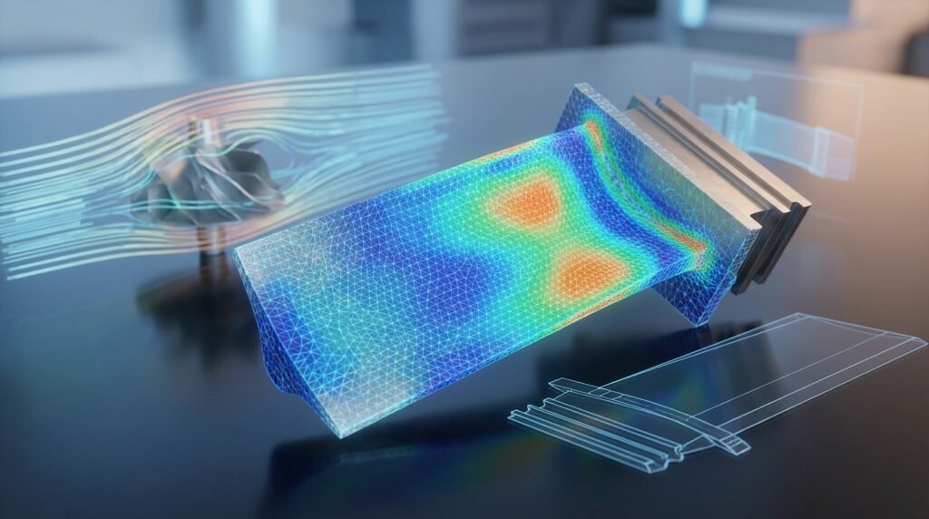
Visualizations: Contour plots (stress, strain, displacement, temperature, pressure), vector plots (flow velocity), deformation plots.
Critical Locations: Identify areas of maximum stress, highest deformation, or potential failure points.
Design Iteration: Use the insights to refine your design, optimize material usage, or improve performance.

FEM in Action: Real-World Engineering Applications

FEM is a versatile tool across countless engineering disciplines.

Structural Engineering & Integrity Assessments

For buildings, bridges, and complex machinery, FEM is indispensable. It’s used to:

Analyze stress and strain distributions under various loading conditions.
Predict deflections and deformations to ensure structural stability.
Perform fatigue life assessments and fracture mechanics (e.g., Fitness-for-Service Level 3 assessments in Oil & Gas).
Evaluate the integrity of pressure vessels, pipelines, and offshore structures.

Aerospace & Automotive Industries

From lightweighting aircraft components to crashworthiness simulations in automotive design, FEM plays a vital role:

Optimizing designs for strength-to-weight ratio.
Analyzing vibrational characteristics and dynamic responses.
Simulating complex impact scenarios using explicit dynamics solvers.

Biomechanics & Medical Devices

FEM helps understand the human body and design better medical solutions:

Analyzing stress in bones and implants.
Simulating the mechanics of soft tissues and organs.
Optimizing prosthetic designs for comfort and durability.

Fluid-Structure Interaction (FSI) & CFD

While often associated with structural analysis, FEM principles extend to Computational Fluid Dynamics (CFD). Furthermore, FSI uses coupled FEM-based solvers (e.g., ANSYS Fluent/Mechanical or OpenFOAM for fluids interacting with structures) to analyze problems like:

Wind loads on structures.
Aeroelasticity of aircraft wings.
Pumping mechanisms and valve performance.

Honing Your FEM Skills: Practical Workflow & Best Practices

Achieving reliable results with FEM requires attention to detail.

1. Mesh Quality is Non-Negotiable

A poor mesh is the fastest way to get unreliable results. Focus on:

Element Shape: Avoid highly distorted elements (e.g., high aspect ratio, excessive skewness).
Refinement: Use finer meshes in regions of high stress gradients, contact zones, or geometric singularities.
Element Order: Linear (first-order) elements are faster but less accurate for bending. Quadratic (second-order) elements provide better accuracy with fewer elements, especially for complex stress states.

2. Accurate Material Models

Ensure your material data accurately reflects the real-world behavior. For advanced simulations:

Consider non-linear material models (plasticity, hyperelasticity for rubber-like materials).
Account for temperature-dependent properties if applicable.
Use anisotropic models for composite materials.

3. Realistic Loads & Boundary Conditions

The problem is only as good as its inputs:

Loading: Apply loads as realistically as possible (e.g., distributed pressure vs. concentrated force).
Constraints: Ensure sufficient constraints to prevent rigid body motion without over-constraining the model.
Contact: Correctly define contact interactions between parts, including friction and separation behavior.

4. Solver Selection & Settings

Different problems require different solvers:

Static vs. Dynamic: Is the problem time-dependent?
Linear vs. Non-linear: Does the material, geometry, or boundary conditions exhibit non-linear behavior? Implicit solvers are generally used for static and quasi-static non-linear problems, while explicit solvers are better for highly dynamic events like impacts.
Convergence: Monitor solver convergence criteria, especially for non-linear analyses, to ensure a stable and accurate solution.

Element Type Comparison (Illustrative)

Element Type	Application	Pros	Cons
Beam (1D)	Slender structures, frames	Fast, efficient	Limited to slender parts, assumes centroidal loading
Shell (2D)	Thin-walled structures (plates, cylinders)	Good for surfaces, captures bending	Assumes thinness, requires mid-surface definition
Solid (3D)	Volumetric components, thick sections	Most general, captures complex stress states	Computationally expensive, mesh generation can be complex

Ensuring Accuracy: Verification & Sanity Checks

Never trust an FEA result blindly. Verification is key to confidence.

1. Convergence Studies

Refine your mesh in critical areas (h-refinement) or increase the element polynomial order (p-refinement) and observe if key results (e.g., maximum stress, deflection) converge to a stable value. This indicates that your solution is mesh-independent.

2. Hand Calculations & Analytical Solutions

For simplified versions of your problem, perform quick hand calculations or use classic engineering formulas (e.g., beam bending equations) to get an order-of-magnitude check on your FEA results. Does the displacement make sense? Is the stress within expected ranges?

3. Sensitivity Analysis

Vary key input parameters (e.g., material properties within their tolerance, load magnitudes, boundary condition locations) and observe the impact on your results. This helps understand the robustness of your design and identifies critical parameters.

4. Check Deformed Shape & Boundary Conditions

Visually inspect the deformed shape of your model. Does it deform as expected? Are your boundary conditions holding as intended? Look for unexpected rigid body motions or overly stiff regions.

5. Reaction Forces & Overall Equilibrium

Sum your reaction forces at constrained boundaries and compare them to the applied loads. They should be in equilibrium (sum to zero) to a very small tolerance. This is a fundamental check.

Navigating Challenges: Common FEM Mistakes & Troubleshooting

Even experienced engineers encounter issues. Here are common pitfalls:

Inadequate Meshing: Too coarse in critical areas leads to inaccurate results; too fine everywhere leads to excessive computation time.
Incorrect Boundary Conditions: Over-constraining (too many restraints) can lead to artificially high stresses. Under-constraining (not enough restraints) results in rigid body motion and solver errors.
Material Property Errors: Wrong units, incorrect values, or inappropriate material models for the given loading conditions.
Contact Setup Issues: Gaps or penetrations between contacting surfaces, or incorrect friction coefficients, can lead to non-convergence or unrealistic contact pressures.
Units Consistency: Always maintain a consistent unit system throughout your model.

Powerful Tools for FEM & Automation

The FEM landscape is rich with powerful software.

Commercial Powerhouses: Abaqus (strong in non-linear and explicit dynamics), ANSYS Mechanical (versatile, comprehensive physics), MSC Nastran/Patran (aerospace, high-performance computing).
CFD Specialists: ANSYS Fluent/CFX, OpenFOAM (open-source, highly customizable).
CAD Integration: Many tools integrate directly with CAD software like CATIA, SolidWorks, and Inventor, streamlining the CAD-CAE workflow.
Automation & Scripting: Python and MATLAB are invaluable for automating repetitive tasks, parametric studies, post-processing results, and even driving software APIs (e.g., Abaqus Python scripting, ANSYS ACT).

Looking to dive deeper into FEM with practical examples or need specialized scripts to automate your workflow? Explore our downloadable templates, projects, and custom Python/MATLAB scripts at EngineeringDownloads.com to accelerate your learning and project delivery.