Rigid Body Motion: Engineering Principles & Simulation

Rigid Body Motion
Engineering Downlaods
April 9, 2026
13 Minute

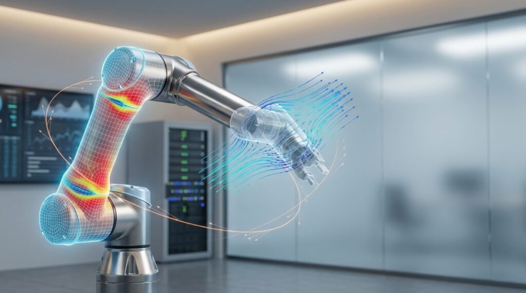
Understanding rigid body motion is fundamental for every engineer involved in mechanical design, robotics, aerospace, or even biomechanics. Imagine designing a robot arm, a vehicle suspension, or analyzing the impact of a falling object. In all these scenarios, the ability to accurately predict how objects move without deforming is absolutely critical. This article will demystify rigid body motion, covering its core concepts, practical applications, and how modern simulation tools help engineers tackle complex challenges.

Image Credit: Cmglee, CC BY-SA 4.0, via Wikimedia Commons

What is Rigid Body Motion?

At its heart, a rigid body is an idealized solid object where deformation is considered negligible. This means that the distance between any two given points within the body remains constant, regardless of external forces or torques applied. When we talk about rigid body motion, we’re describing how such an object moves through space.

This simplification is incredibly powerful because it allows engineers to focus on the overall kinematics (motion without considering forces) and kinetics (motion considering forces and torques) of complex systems without getting bogged down by intricate material deformation, which would require much more computational effort.

Key Concepts: Translation & Rotation

Any general motion of a rigid body can be decomposed into two primary types:

Translational Motion

Definition: Every point within the rigid body moves along parallel paths. The body does not rotate.
Characteristics: All points have the same velocity and acceleration at any given instant.
Parameters: Described by linear displacement, velocity, and acceleration. These are typically vector quantities.
Example: A car moving in a straight line, a block sliding on a surface.

Rotational Motion

Definition: The rigid body moves such that all points trace circular paths about a fixed axis of rotation. This axis can be internal or external to the body.
Characteristics: Points further from the axis of rotation have higher linear velocities, but all points share the same angular velocity and angular acceleration.
Parameters: Described by angular displacement, angular velocity (ω), and angular acceleration (α). These are also vector quantities.
Example: A spinning wheel, a door opening on its hinges.

Most real-world rigid body motion is a combination of both translation and rotation. Think of a rolling wheel or a rocket performing maneuvers in flight – both are simultaneously translating and rotating.

Why is Rigid Body Motion Crucial for Engineers?

The principles of rigid body motion are the bedrock for designing, analyzing, and optimizing a vast array of engineering systems. Here are a few reasons why it’s indispensable:

Mechanism Design: From simple linkages to complex robotic arms, understanding how components move relative to each other is key to ensuring functionality and avoiding interference.
Vehicle Dynamics: Analyzing the ride and handling of cars, aircraft, and spacecraft relies heavily on rigid body dynamics to model suspension systems, control surfaces, and overall stability.
Impact Analysis: While severe impacts cause deformation, initial contact and overall body trajectories can often be modeled effectively using rigid body assumptions.
Biomechanics: Understanding human joint movement, gait analysis, and prosthetic design often begins with treating bones and limbs as rigid bodies.
Manufacturing Automation: Designing automated assembly lines, pick-and-place robots, and material handling systems requires precise control over rigid body kinematics and kinetics.

Analyzing Rigid Body Motion: Tools & Techniques

Engineers employ a range of methods, from classical hand calculations to sophisticated simulation software, to analyze rigid body motion.

Manual Calculations: The Foundation

Before diving into software, a solid grasp of manual calculation techniques is essential. These include:

Newton-Euler Equations: Applying Newton’s second law for linear motion and Euler’s equations for rotational motion. This approach is fundamental.
Lagrangian Mechanics: A powerful energy-based approach that can simplify the derivation of equations of motion for complex multi-body systems, especially useful when dealing with constraints.
Kinematic Chains: Using vector loops and rotation matrices to determine positions, velocities, and accelerations of points in a system of interconnected rigid bodies.

While manual calculations are vital for understanding and basic checks, they become prohibitively complex for systems with many bodies, joints, and dynamic interactions.

Simulation Software (MBD/FEA)

For more intricate problems, dedicated simulation tools are indispensable. These can broadly be categorized into Multi-Body Dynamics (MBD) software and Finite Element Analysis (FEA) software with rigid body capabilities.

Multi-Body Dynamics (MBD) Software

MBD software is purpose-built for systems composed of multiple interconnected rigid or flexible bodies. They excel at simulating kinematic and dynamic behavior, reaction forces, and joint loads. Key features include:

Joint Libraries: Extensive pre-defined joints (revolute, prismatic, spherical, universal, etc.) that accurately represent mechanical connections.
Force Elements: Easy application of springs, dampers, bushings, and contact forces.
Solver Efficiency: Optimized for solving the coupled equations of motion for many bodies, often using techniques like Lagrange multipliers or recursive formulations.
Common Tools: MSC ADAMS, Simscape Multibody (MATLAB), RecurDyn.

Implicit vs. Explicit FEA for Rigid Body Dynamics

While FEA primarily deals with deformation, it can be used for rigid body motion, particularly when contact is critical or localized deformation might occur at interfaces. FEA solvers allow you to define parts as ‘rigid’ to save computational cost while still capturing their global motion and interactions.

Implicit FEA: Generally suitable for static or quasi-static problems. For rigid body dynamics, it can be used for slower-moving contact problems, but often struggles with highly transient or impact events due to stability requirements and small time steps.
Explicit FEA: The preferred choice for high-speed dynamics, impacts, and highly non-linear contact problems. Solvers like Abaqus/Explicit and ANSYS Explicit Dynamics are excellent for modeling rigid body contact and impact, as they use small, stable time steps that propagate disturbances explicitly. Even if a body is declared rigid, the solver still tracks its motion and interactions efficiently.

Feature	MBD Software (e.g., ADAMS)	FEA Software (e.g., Abaqus/Explicit)
Primary Focus	Kinematics & Dynamics of interconnected bodies	Stress, strain, deformation, failure
Body Definition	Treats bodies as inherently rigid (or flexible for MBD with flexibility)	Allows declaration of parts as rigid (or deformable)
Complexity of Contact	Good for general contact, basic friction, complex joint interactions	Excellent for complex, highly nonlinear contact, friction, impacts, detailed contact stresses
Computational Cost	Generally lower for large systems of discrete bodies	Higher, especially for deformable bodies; lower for truly rigid parts
Typical Use Cases	Mechanism design, vehicle dynamics, robotics, joint loads	Impact analysis, crashworthiness, fluid-structure interaction with rigid parts, complex contact
Material Properties	Mass, inertia, CoG; often less focus on elastic properties unless flexible bodies are used	Full material models (elastic, plastic, hyperelastic, etc.) for deformable parts; mass & inertia for rigid parts

Practical Workflow: Simulating Rigid Body Motion

Here’s a generalized workflow for analyzing rigid body motion using simulation software, applicable to both MBD and FEA contexts:

Step-by-Step Guide

1. Define the System & Objectives

Identify Components: List all rigid bodies, their degrees of freedom (DoF), and how they interact.
Establish Goals: What do you want to achieve? (e.g., joint forces, velocities, accelerations, overall trajectory, impact forces).
Simplify: Determine if any parts can be ignored or simplified. For example, treating a complex assembly as a single rigid body if only its global motion matters.

2. Model Creation

CAD Import: Bring in your CAD geometry (e.g., from CATIA, SolidWorks).
Mass & Inertia: Assign correct mass, center of gravity (CoG), and moments of inertia to each rigid body. These are critical for accurate dynamic response.

3. Material Properties & Connections

Material Properties: For ‘rigid’ parts, you primarily need density to calculate mass and inertia. For contact surfaces, friction coefficients are crucial.
Joints & Constraints: Define all mechanical connections (revolute, prismatic, fixed, etc.) accurately. This is where MBD software shines. For FEA, kinematic couplings or constraints mimic joints.
Contact Definitions: Specify contact interactions between bodies, including contact algorithms, friction, and potentially impact parameters (e.g., coefficient of restitution).

4. Loads & Boundary Conditions

Applied Forces/Torques: Define external forces, gravity, spring forces, motor torques, or prescribed motions.
Boundary Conditions (BCs): Fix certain DoF (e.g., a fixed pivot point) or apply initial conditions (e.g., initial velocity).

5. Solver Setup & Execution

Solver Selection: Choose the appropriate solver (e.g., explicit dynamics for impact, implicit for quasi-static multi-body).
Time Step: Define the total simulation time and appropriate time step. For explicit solvers, stability is often automatically handled, but for implicit, careful choice is needed.
Output Requests: Specify what results you need (e.g., time histories of velocities, accelerations, forces, energies).

Need help setting up your rigid body simulations in Python or MATLAB? EngineeringDownloads.com offers specialized tutoring and downloadable script templates to accelerate your learning and project delivery.

6. Post-Processing & Interpretation

Visualize Motion: Animate the results to visually confirm the expected behavior.
Plot Results: Extract and plot quantities like joint forces, velocities, accelerations over time.
Analyze Data: Compare simulation results against design requirements, experimental data, or hand calculations.

Verification & Sanity Checks

Rigid body simulations, while less prone to mesh dependency than full FEA, still require rigorous verification:

Units Consistency: Ensure all inputs (mass, length, time, force) are in a consistent unit system. This is a common source of error.
Conservation of Energy: For conservative systems, total mechanical energy (kinetic + potential) should be conserved or only dissipate through friction/damping. Monitor energy plots.
Boundary Condition Review: Double-check that all constraints and loads are applied correctly and logically. Does a fixed joint truly represent the physical connection?
Simplified Hand Calculations: For a very simplified case (e.g., a single rigid body under gravity), perform a quick hand calculation to benchmark the simulation’s output.
Parameter Sensitivity: Run simulations with slightly varied parameters (e.g., friction coefficients, joint stiffness) to understand their impact and ensure your results are robust.
Convergence: For MBD solvers, ensure the solver achieves convergence at each time step, indicating a stable and accurate solution.

Common Pitfalls & Troubleshooting

Incorrect Joint Definitions: Misdefining a joint (e.g., using a fixed joint instead of a revolute) can lead to non-physical motion or over-constraints.
Unrealistic Contact Parameters: Too high or too low friction, or incorrect contact stiffness settings, can cause bodies to penetrate or bounce excessively.
Numerical Instability: Especially in explicit dynamics, overly large time steps or highly stiff contact can cause oscillations or ‘explosions’. Adjust time steps or contact algorithms.
Mass & Inertia Errors: Incorrectly entered mass or moments of inertia will fundamentally alter dynamic response. Always verify these against CAD properties.
Over-Constrained Systems: Applying redundant constraints can lead to solver errors or incorrect reaction forces. Carefully check for conflicting boundary conditions.
Gravity Direction: A simple mistake, but applying gravity in the wrong direction or neglecting it when it’s significant.

Best Practices for Accurate Analysis

Start Simple: Begin with a simplified model and gradually add complexity.
Validate Against Known Data: If possible, compare simulation results against experimental data or analytical solutions for similar problems.
Document Assumptions: Clearly state all assumptions made (e.g., truly rigid bodies, frictionless joints).
Perform Sensitivity Studies: Understand how changes in input parameters affect your results.
Collaborate: Discuss your models and results with colleagues for fresh perspectives.