Demystifying CFD Principles: A Practical Engineer’s Guide
Computational Fluid Dynamics (CFD) is a powerful simulation tool that allows engineers to predict fluid flow, heat transfer, and related phenomena. From designing more aerodynamic aircraft to optimizing complex piping systems in oil & gas, CFD is indispensable. But beyond the flashy visualizations, understanding the core CFD principles is what truly empowers you to perform accurate and reliable analyses.
This article cuts through the academic jargon to provide a practical, engineer-to-engineer understanding of CFD. We’ll cover everything from the fundamental equations to real-world workflow tips and crucial verification steps.

Image: Illustrative CFD simulation showing streamlines around an airfoil.
The Core Pillars of CFD: Building Your Simulation Foundation
At its heart, CFD solves a set of mathematical equations that describe fluid motion. Let’s break down the essential components.
Governing Equations: The Language of Fluid Motion
CFD is fundamentally built upon the conservation laws of physics:
- Conservation of Mass (Continuity Equation): States that mass cannot be created or destroyed. For a steady flow, the mass entering a control volume must equal the mass leaving it.
- Conservation of Momentum (Navier-Stokes Equations): These are Newton’s second law applied to fluid motion, describing the balance between forces (pressure, viscous, gravity) and the acceleration of fluid particles.
- Conservation of Energy (Energy Equation): Accounts for heat transfer phenomena like conduction, convection, and radiation, crucial for thermal analysis in aerospace or biomechanics applications.
These equations, often complex and non-linear, are typically solved numerically.
Eulerian vs. Lagrangian Perspective
- Eulerian Approach: Focuses on fluid properties at fixed points in space as fluid flows through them (e.g., measuring velocity at a specific sensor location). Most traditional CFD solvers (Fluent, OpenFOAM) use this.
- Lagrangian Approach: Follows individual fluid particles or elements as they move through the flow field (e.g., Discrete Phase Model for particle tracking).
Discretization Methods: Turning Equations into Computable Problems
Since we can’t solve the governing equations analytically for most real-world problems, we discretize them. This involves dividing the continuous fluid domain into a finite number of discrete elements or volumes.
Finite Volume Method (FVM)
The most common method in commercial CFD software (ANSYS Fluent/CFX, OpenFOAM). It involves:
- Dividing the domain into small, non-overlapping control volumes.
- Integrating the governing equations over each control volume.
- Approximating flux terms at the control volume faces using interpolation schemes.
Takeaway: FVM conserves mass, momentum, and energy on a discrete level, making it robust.
Finite Element Method (FEM)
Widely used in structural analysis (FEA tools like Abaqus, ANSYS Mechanical) and gaining traction in CFD for complex geometries and unstructured meshes. It works by:
- Dividing the domain into elements.
- Approximating the solution within each element using shape functions.
- Formulating a system of equations that are solved simultaneously.
Finite Difference Method (FDM)
Historically significant, FDM approximates derivatives in the governing equations using differences between nodal values. It’s simpler to implement but less flexible for complex geometries, typically restricted to structured grids.
Meshing: The Foundation of Any Simulation
The mesh (or grid) is a discrete representation of your fluid domain. Its quality profoundly impacts simulation accuracy and computational cost.
Mesh Types
- Structured Mesh: Regular, organized grid with identifiable i, j, k directions. High quality, efficient for simple geometries, but hard to generate for complex shapes.
- Unstructured Mesh: Irregular grid (e.g., triangles, tetrahedra). Flexible for complex geometries, common in industrial applications.
- Hybrid Mesh: Combines structured and unstructured regions, often used for efficiency in specific areas like boundary layers.
Mesh Quality Considerations
A good mesh is:
- Orthogonal: Cell faces are perpendicular to cell edges.
- Smoothly Varying: Cell size changes gradually.
- Low Aspect Ratio: Cells are not excessively stretched (e.g., long and thin).
- Refined in Key Areas: Denser near walls, wakes, and high-gradient regions (e.g., around an airfoil in aerospace applications, or near a valve in oil & gas).
Poor mesh quality can lead to divergence, inaccurate results, and excessive computational time.
Boundary Conditions (BCs) and Initial Conditions (ICs)
These define the interaction of your fluid domain with its surroundings and its starting state.
Common BC Types
- Inlet: Specifies velocity, pressure, temperature, or mass flow rate.
- Outlet: Specifies pressure (e.g., atmospheric pressure) or outflow conditions.
- Wall: Defines no-slip (velocity is zero relative to the wall) or slip conditions, and thermal conditions (adiabatic, constant temperature, heat flux).
- Symmetry: Used to model a portion of a symmetric geometry, reducing computational cost.
- Periodic: For flows that repeat spatially (e.g., turbomachinery blades).
Importance of ICs
For transient (time-dependent) simulations, initial conditions are crucial. For steady-state problems, a reasonable initial guess can accelerate convergence, but the final solution shouldn’t depend on it.
Solvers and Numerical Schemes
After discretization, the governing equations transform into a system of algebraic equations. The solver’s job is to solve these equations.
Pressure-Velocity Coupling
A major challenge in incompressible flows is that pressure doesn’t have an explicit governing equation. Algorithms like SIMPLE (Semi-Implicit Method for Pressure-Linked Equations) and PISO (Pressure-Implicit with Splitting of Operators) are used to iteratively couple pressure and velocity fields.
Temporal Discretization (for Transient Simulations)
- Explicit Schemes: Solution at a new time step depends only on known values at the current time step. Simpler but often require very small time steps for stability.
- Implicit Schemes: Solution at a new time step depends on values at both the current and new time steps. More computationally intensive per time step but allow larger time steps, offering better stability.
Practical CFD Workflow: From CAD to Insights
Performing a successful CFD simulation involves a structured approach. Here’s a typical workflow:
Step 1: Problem Definition
Clearly define your objectives. What do you want to achieve? What are the key performance indicators (KPIs)? What fluid phenomena are important? (e.g., pressure drop across a valve, heat transfer in a heat exchanger, lift on an aircraft wing).
Step 2: Geometry Preparation
Start with your CAD model (e.g., created in CATIA, SolidWorks). For CFD, you’ll need the fluid domain, not the solid part. This often involves creating an enclosure around or inside your solid geometry. Simplify the geometry by removing small features (fillets, bolts) that are computationally expensive but don’t significantly impact the overall flow physics.
Step 3: Mesh Generation
This is often the most time-consuming step. Use meshing tools (e.g., ANSYS Meshing, OpenFOAM’s snappyHexMesh, Salome) to create a high-quality mesh. Pay special attention to boundary layers near walls to accurately capture viscous effects. Consider doing a preliminary mesh study to determine appropriate cell sizes.
Step 4: Setting Up the Physics
In your CFD solver (e.g., ANSYS Fluent, CFX, OpenFOAM), you’ll:
- Select the appropriate fluid properties (density, viscosity).
- Choose a suitable turbulence model (more on this later).
- Define boundary conditions (inlets, outlets, walls, symmetry planes).
- Specify initial conditions (for transient simulations).
- Set up solver controls (e.g., under-relaxation factors, convergence criteria).
Step 5: Solving
Run the simulation. Monitor residuals (a measure of how well the equations are satisfied) to ensure convergence. For transient simulations, monitor key output variables over time.
Step 6: Post-Processing and Visualization
This is where you extract insights. Use post-processing tools (e.g., ParaView, ANSYS CFD-Post) to:
- Visualize flow fields (velocity vectors, streamlines, contours of pressure/temperature).
- Generate plots of relevant quantities (e.g., pressure drop, heat transfer rate, drag/lift coefficients).
- Create animations for transient flows.
This stage is crucial for understanding the fluid behavior and making informed engineering decisions.
Verification & Sanity Checks in CFD
A fancy visualization is useless if it’s not accurate. Always perform rigorous checks.
Mesh Independence Study
Run your simulation with at least three different mesh densities (coarse, medium, fine). If your results (e.g., pressure drop, average velocity) change significantly between the medium and fine meshes, your mesh is not sufficiently refined. This is a critical step for ensuring your solution is independent of the mesh.
Convergence Monitoring
Ensure that the residuals drop to sufficiently low levels (e.g., 10-4 to 10-6 for most equations). Also, monitor key engineering quantities (like lift, drag, pressure drop) to ensure they reach a steady state or a stable oscillation for transient problems. If these quantities are still changing, your simulation hasn’t converged, regardless of residual values.
Physical Plausibility Checks
- Flow Direction: Does fluid flow as expected (e.g., from high pressure to low pressure)?
- Velocity/Pressure Profiles: Do profiles look reasonable (e.g., parabolic profile in a pipe, boundary layer growth)?
- Conservation: Is mass, momentum, and energy conserved across your domain (e.g., inflow mass equals outflow mass)?
- Extreme Values: Are there any unphysical velocities, pressures, or temperatures? These often indicate mesh errors or poor boundary conditions.
Validation: Comparing with Experiments/Analytics
Whenever possible, validate your CFD model against experimental data or known analytical solutions. This builds confidence in your model’s predictive capabilities. For example, validating pressure drop predictions against published data for a specific pipe geometry.
Sensitivity Analysis
How sensitive are your results to input parameters (e.g., material properties, boundary condition values)? Performing a sensitivity analysis helps understand the robustness of your design and simulation.
Common Pitfalls and Troubleshooting
- Divergence: Often caused by poor mesh quality, incorrect boundary conditions, or aggressive solver settings. Start by checking mesh and BCs, then reduce under-relaxation factors or use smaller time steps.
- Slow Convergence: Can be due to complex physics, poor mesh, or numerical instability. Try different solver schemes or initial conditions.
- Unphysical Results: Always question results that don’t make sense. Re-check your inputs, units, and model setup thoroughly.
Turbulence Modeling: A Critical Aspect of Many Flows
Most real-world fluid flows are turbulent, characterized by chaotic, unsteady motion. Modeling turbulence directly (Direct Numerical Simulation – DNS) is computationally prohibitive for most engineering problems.
RANS Models (Reynolds-Averaged Navier-Stokes)
The most widely used approach. RANS models average the Navier-Stokes equations over time, introducing additional terms (Reynolds stresses) that need to be modeled. Popular RANS models include:
| Model Name | Key Characteristics | Typical Applications |
|---|---|---|
| k-epsilon | Robust, widely used, good for many industrial flows, can struggle with adverse pressure gradients. | Pipes, ducts, simple external aerodynamics, general industrial flows. |
| k-omega (SST) | Good for boundary layers, adverse pressure gradients, and separation. Blends k-epsilon in free stream and k-omega near walls. | Aerospace (airfoils, wings), turbomachinery, external aerodynamics. |
| Spalart-Allmaras | Economical, good for external aerodynamics, especially in aerospace. Primarily for wall-bounded flows. | Aircraft design, vehicle aerodynamics. |
| Reynolds Stress Model (RSM) | Most complex RANS model, directly solves for Reynolds stresses, better for complex 3D flows with strong swirling or anisotropy. | Cyclone separators, swirling flows, highly anisotropic flows. |
LES and DNS
- Large Eddy Simulation (LES): Resolves large turbulent eddies directly and models smaller eddies. More accurate than RANS but significantly more computationally expensive.
- Direct Numerical Simulation (DNS): Resolves all scales of turbulence down to the Kolmogorov microscale. Extremely accurate but prohibitively expensive for most engineering applications, used primarily for fundamental research.
Applications of CFD Across Industries
CFD is a versatile tool, finding applications in diverse fields:
- Aerospace: Aircraft and rocket design (drag, lift, thermal management), jet engine performance.
- Automotive: Vehicle aerodynamics, engine combustion, thermal management, HVAC.
- Oil & Gas: Pipeline flow, offshore platform hydrodynamics, multiphase flow in risers, fluid-structure interaction (FFS Level 3 assessments).
- Biomechanics: Blood flow in arteries, prosthetic device design, drug delivery.
- HVAC: Building ventilation, cleanroom design, thermal comfort.
- Process Engineering: Mixer design, reactor optimization, heat exchanger performance.
Leveraging Automation: Python & MATLAB in CFD Workflows
Modern engineering demands efficiency. Python and MATLAB are invaluable for automating various stages of CFD:
- Pre-processing: Generating parametric geometries, automating mesh generation inputs, creating complex boundary conditions, and scripting solver setup files.
- Post-processing: Extracting specific data, creating custom plots, automating report generation, and performing statistical analysis on results.
- Parametric Studies & Optimization: Running multiple simulations with varying design parameters to optimize performance (e.g., wing shape optimization, pipe diameter sizing).
Many commercial CFD packages offer API access for scripting, making integration seamless.
Ready to Dive Deeper?
Mastering CFD takes practice. If you’re looking for hands-on experience, advanced tutorials, or custom scripts for your ANSYS Fluent, OpenFOAM, or Python-based CFD projects, explore the downloadable resources and online consultancy options at EngineeringDownloads.com. We offer tailored support to help you tackle your toughest fluid dynamics challenges.
Further Reading
For more in-depth information on specific CFD topics, consider exploring the official documentation and learning resources provided by leading CFD software vendors like ANSYS: What is CFD? – ANSYS Blog