Abaqus stands as a cornerstone in the world of advanced engineering simulation, a powerful suite of Finite Element Analysis (FEA) tools from Dassault Systèmes’ SIMULIA portfolio. For engineers tackling complex structural, thermal, and multiphysics problems, Abaqus offers robust capabilities for highly nonlinear behavior, large deformations, and intricate contact interactions. This guide dives into the practical aspects of using Abaqus, designed for engineers who need clear, actionable insights to enhance their simulation proficiency.

Courtesy of Wikimedia Commons.
Why Abaqus? The Engineer’s Edge
Abaqus is more than just an FEA solver; it’s a comprehensive platform. Its strength lies in its versatility and advanced material modeling capabilities, making it indispensable across various industries.
- Broad Capabilities: From static stress analysis to complex dynamic events, thermal-mechanical coupling, acoustics, and even coupled Eulerian-Lagrangian (CEL) analyses for fluid-structure interaction.
- Nonlinear Prowess: Excelles in handling material nonlinearity (plasticity, hyperelasticity, creep), geometric nonlinearity (large deformations, buckling), and contact nonlinearity.
- Industry Adoption: Widely used in aerospace for airframe integrity, in oil & gas for pipeline analysis and structural integrity (FFS Level 3 assessments), in biomechanics for medical device design, and in automotive for crashworthiness and durability.
- Advanced Materials: Strong support for composites, rubber, foam, and even user-defined material models (UMAT/VUMAT).
Abaqus Core Modules: A Quick Tour
The Abaqus suite comprises several modules, each tailored for specific analysis types and workflows:
- Abaqus/Standard: The implicit solver, ideal for static, low-speed dynamic, and quasi-static problems where equilibrium is sought incrementally. It’s excellent for processes with long event durations or requiring detailed stress distribution.
- Abaqus/Explicit: The explicit dynamic solver, designed for highly nonlinear transient problems such as impact, crashworthiness, blast simulations, and manufacturing processes involving large deformations. It’s computationally efficient for short-duration events.
- Abaqus/CAE (Complete Abaqus Environment): The graphical user interface (GUI) for pre-processing (model creation, meshing, boundary conditions) and post-processing (results visualization and interpretation). It streamlines the entire simulation workflow.
- Abaqus/Viewer: A dedicated post-processor for viewing results from Abaqus/Standard and Abaqus/Explicit output databases.
Practical Workflow in Abaqus: A Step-by-Step Approach
A successful Abaqus simulation follows a methodical approach. Here’s a typical workflow you’ll encounter:
1. Pre-processing: Setting Up Your Model
This is where you build the digital twin of your physical system.
- CAD Import & Geometry Cleanup:
- Import geometry (STEP, IGES, Parasolid are common).
- Clean up imperfections: remove small faces, sliver edges, or redundant features that can complicate meshing. Simplify complex geometry where appropriate to reduce computational cost.
- Material Definition:
- Define material properties: Young’s modulus, Poisson’s ratio for linear elasticity.
- For nonlinear behavior, add plasticity data (stress-strain curves), hyperelastic parameters (Mooney-Rivlin, Ogden for rubber), or creep laws. Ensure units are consistent!
- Meshing Strategies:
- Choose appropriate element types (e.g., C3D8R for 3D solids, S4R for shells).
- Apply global and local mesh seeds. Refine mesh in areas of high-stress gradients or critical contact zones.
- Prioritize hexahedral meshes where possible for accuracy and efficiency, but tetrahedral meshes are often necessary for complex geometries.
- Boundary Conditions & Loads:
- Apply constraints (fixed, pinned, symmetry conditions) to restrict rigid body motion.
- Define loads: pressure, concentrated forces, moments, prescribed displacements, or thermal loads.
- Ensure that your boundary conditions accurately reflect the real-world constraints on your component.
- Interaction Properties:
- Define contact pairs or general contact. Specify friction coefficients.
- Define connections (e.g., ties, fasteners, rigid body constraints) between different parts of your assembly.
2. Job Submission & Monitoring
Once your model is defined, it’s time to run the analysis.
- Creating and Submitting a Job: In Abaqus/CAE, create a ‘Job’ instance, selecting the model, analysis type (Standard or Explicit), and computational resources (processors, memory). Submit the job.
- Monitoring Progress: Keep an eye on the job monitor for warnings, errors, and convergence issues. Review the .dat and .msg files for detailed information, especially if the job aborts or fails to converge.
3. Post-processing: Interpreting Results
Extracting meaningful data from your simulation is crucial.
- Visualization & Plotting: View deformed shapes, stress contours (Von Mises, principal stresses), strain, displacement, and reaction forces. Use section cuts to inspect internal stress states.
- Querying Results: Use the query tools to get specific values at nodes/elements, along paths, or for entire regions.
- Reporting: Generate plots, animations, and tables of critical results for documentation and design review.
Key Considerations for Robust Simulations
Achieving reliable results with Abaqus requires attention to detail in several key areas.
Material Modeling: Beyond Linear Elasticity
Many real-world engineering problems involve materials exhibiting nonlinear behavior. Ignoring this can lead to inaccurate predictions.
- Plasticity: For metals loaded beyond their yield point. Ensure you have accurate stress-strain data from material tests.
- Creep: Time-dependent deformation under constant stress, critical for high-temperature applications.
- Hyperelasticity: For rubber-like materials. Choosing the correct constitutive model (e.g., Ogden, Arruda-Boyce) based on experimental data is vital.
- Fracture Mechanics: Abaqus supports advanced techniques like eXtended Finite Element Method (XFEM) for crack initiation and propagation, or cohesive zone modeling (CZM) for delamination studies.
Contact Analysis: Getting It Right
Contact is a frequent source of convergence issues and incorrect results if not set up carefully.
- Types of Contact: Abaqus offers ‘Surface-to-surface’ contact (more robust for general cases) and ‘Node-to-surface’ contact (often used with rigid surfaces). ‘General contact’ simplifies setup for complex assemblies but requires careful tuning.
- Friction Models: Define coefficients of friction for tangential behavior. Consider if ‘rough’ contact (no relative slip) or ‘sticky’ contact (cohesion) is appropriate.
- Common Pitfalls: Overclosure (initial penetration), high contact stiffness leading to oscillation, and insufficient stabilization methods can all cause problems. Use contact stabilization and adjust contact controls as needed.
Dynamic Simulations: Standard vs. Explicit
Choosing the right solver is paramount for dynamic problems.
- Abaqus/Standard (Implicit): Suitable for problems where inertial effects are moderate, and dynamic equilibrium is maintained incrementally. Think modal analysis, steady-state dynamics, or impact where the event duration is relatively long and damping is significant.
- Abaqus/Explicit (Explicit): Ideal for highly transient, short-duration events like impact, crash, blast, or severe forming operations. It handles large distortions and complex contact more robustly. The stability limit for the time increment is crucial for accurate results.
Verification & Sanity Checks: Ensuring Accuracy
Never trust a simulation result blindly. Rigorous verification and validation are critical.
- Mesh Sensitivity Analysis: Run your analysis with progressively finer meshes. Results should converge to a stable value. If not, your mesh might still be too coarse or element quality is poor.
- Convergence Criteria: For Abaqus/Standard, monitor the force and moment equilibrium during iterations. Non-convergence often indicates issues with boundary conditions, material properties, or contact definitions.
- Boundary Condition Impact: Slightly perturb your boundary conditions to assess their influence. Are the results overly sensitive to minor changes?
- Analytical/Hand Calculation Comparisons: For simplified cases or sub-regions of your model, compare Abaqus results to theoretical solutions or basic hand calculations. This builds confidence in your model’s fundamental behavior.
- Sensitivity Studies: Vary key input parameters (e.g., material stiffness, load magnitude) within their expected ranges to understand how they affect the output.
- Common Troubleshooting Scenarios:
- Non-convergence: Check for rigid body motion, highly distorted elements, sudden contact changes, or material instabilities.
- High Energy Errors (Explicit): Indicates excessive artificial energy; check time step, element quality, and mass scaling if applied.
- Singularities: Often at sharp corners or point loads. Understand that these are mathematical and not always physically realistic.
Automating Abaqus with Scripting
Abaqus provides a powerful Python-based scripting interface (Abaqus Scripting Interface, ASI) that allows you to automate tasks, build parametric models, and customize post-processing.
- Python Scripting: Every action you perform in Abaqus/CAE is recorded in a Python script (the ‘journal file’). This is an excellent starting point for understanding how to script.
- Common Automation Tasks:
- Creating parametric models to study design variations.
- Automating repetitive pre-processing steps.
- Extracting specific results and generating custom reports.
- Running multiple jobs in batch mode.
For advanced Python scripting templates or custom automation solutions, explore EngineeringDownloads.com’s resources. We offer expert tutoring and online consultancy to help optimize your Abaqus workflows.
Integration with CAD/CAE Ecosystem
Abaqus doesn’t operate in a vacuum. Its ability to integrate with other engineering tools enhances its utility.
- CAD Integration: Direct connectors exist for popular CAD software like CATIA, SolidWorks, and Inventor, allowing seamless transfer of geometry.
- Coupling with CFD Tools: For complex Fluid-Structure Interaction (FSI) problems, Abaqus can be coupled with Computational Fluid Dynamics (CFD) software (e.g., ANSYS Fluent or OpenFOAM) through co-simulation interfaces.
- Data Exchange: Exporting/importing data in universal formats like IGES, STEP, or even direct FEA data like Nastran bulk data files facilitates interoperability with other FEA packages (e.g., MSC Patran/Nastran).
Abaqus vs. Other FEA Solvers: A Brief Comparison
While Abaqus is a leader, understanding its position relative to other major FEA tools is helpful.
| Feature/Software | Abaqus (SIMULIA) | ANSYS Mechanical | MSC Nastran |
|---|---|---|---|
| Strength | Nonlinear, Contact, Advanced Materials, Multiphysics | User-friendly GUI, Broad physics portfolio, Robust linear/nonlinear | Linear static/dynamic, Aerospace industry standard, High performance |
| Primary Solvers | Standard (Implicit), Explicit (Explicit) | Mechanical APDL (MAPDL), Workbench Solvers | SOL 101, 103, 108, 400 etc. |
| Usability | Powerful CAE GUI, Python scripting | Workbench (GUI), APDL scripting | Primarily input file driven (pre-processors like Patran are common) |
| Industries | Aerospace, O&G, Automotive, Biomechanics, Advanced Research | Aerospace, Automotive, Energy, Electronics, Civil | Aerospace, Automotive, Heavy Industry |
| Key Differentiator | Deep nonlinear and explicit capabilities, advanced material models | Integrated multidisciplinary platform, strong CAD/CAE workflow | Legacy for linear analysis, certification in aerospace, high performance for large models |
Best Practices Checklist for Abaqus Users
Follow these guidelines for more efficient and reliable simulations:
- ✓ Start Simple: Begin with a simplified model (e.g., linear, no contact) to establish a baseline before adding complexity.
- ✓ Units Consistency: Always use a consistent system of units throughout your model (e.g., mm, N, MPa, s).
- ✓ Review Warnings: Don’t ignore warnings in the .msg or .dat files; they often point to potential issues.
- ✓ Element Quality: Prioritize good element aspect ratios, skewness, and Jacobian values, especially in critical areas.
- ✓ Small Displacement vs. Large Displacement: Understand when to activate geometric nonlinearity (NLGEOM) based on expected deformation.
- ✓ Backup Regularly: Save your model frequently and in different iterations.
- ✓ Document Your Work: Keep notes on assumptions, material sources, and analysis choices.
Common Mistakes and How to Avoid Them
- Incorrect Units: A perpetual problem. Always double-check your unit system for geometry, material properties, and loads.
- Poor Mesh Quality: Leading to inaccurate stress concentrations or convergence difficulties. Invest time in mesh refinement and element quality checks.
- Ill-Defined Boundary Conditions: Over-constraining or under-constraining the model can lead to unrealistic results or rigid body motion. Ensure proper restraints for all six degrees of freedom if necessary.
- Ignoring Contact Set-up: Incorrect contact definitions (e.g., no friction when it’s present, using inappropriate contact algorithms) is a leading cause of non-convergence.
- Material Property Errors: Using generic material properties instead of tested data, or inputting properties incorrectly (e.g., shear modulus instead of Young’s).
- Over-Complicating Initial Models: Jumping straight to highly nonlinear, complex models without understanding the basics first. Incrementally add complexity.
Further Reading / Reference
Dassault Systèmes SIMULIA Abaqus Product Page