When diving into Finite Element Analysis (FEA) or Computational Fluid Dynamics (CFD), achieving accurate results often hinges on the quality of your mesh. One critical aspect that frequently dictates success, especially for analyses involving fluid flow or contact phenomena, is the strategic use of inflation layers. These specially crafted mesh elements are paramount for capturing steep gradients near boundaries, ensuring your simulations truly reflect the underlying physics.
Understanding and correctly implementing inflation layers can make the difference between a convergent, accurate simulation and one riddled with errors or misleading data. This guide will walk you through the ‘why,’ ‘what,’ and ‘how’ of inflation layers, arming you with the practical knowledge to elevate your engineering simulations.

Illustrative example of mesh refinement near a boundary, highlighting the concept of inflation layers.
What are Inflation Layers and Why Do They Matter?
Inflation layers, also known as boundary layer meshes or prismatic layers, are thin, extruded mesh elements intentionally placed adjacent to fluid-solid interfaces or structural contact surfaces. Their primary purpose is to resolve the steep gradients of velocity, temperature, pressure, or stress that occur within the boundary layer – a region where viscous or contact effects dominate.
The Critical Role in CFD
In CFD, capturing the boundary layer accurately is non-negotiable for predicting wall shear stress, heat transfer rates, flow separation, and pressure drop. Without adequate resolution provided by inflation layers, turbulence models (especially RANS models), and near-wall physics cannot be correctly computed, leading to significant errors in drag, lift, heat flux, and overall flow behavior.
Importance in FEA and Structural Integrity
While often associated with CFD, inflation layers also have relevance in specific FEA applications. For instance, in contact mechanics, highly refined elements near contact surfaces can be crucial for accurately capturing stress concentrations and contact pressures. Similarly, in Fracture Mechanics (FFS Level 3 assessments), a fine mesh transition near crack tips or stress raisers, conceptually similar to boundary layer refinement, is essential for precise stress intensity factor calculations.
The Science Behind Effective Inflation Layers
The effectiveness of inflation layers stems from their ability to place computational points precisely where the physics changes most rapidly. This high density of elements near the wall ensures that numerical schemes can accurately interpolate and solve for variables in these critical regions.
Boundary Layer Theory Fundamentals
- Fluid Mechanics: The no-slip condition at the wall creates a velocity gradient from zero at the surface to the freestream velocity further away. This thin region is the boundary layer.
- Heat Transfer: Similarly, a thermal boundary layer forms when there’s a temperature difference between the fluid and the wall.
- Turbulence: In turbulent flows, the boundary layer is complex, often divided into a viscous sublayer, buffer layer, and logarithmic layer. Resolving these layers is critical for turbulence model accuracy.
Introducing y+ and Its Significance
For turbulent flows, the dimensionless wall distance, y+, is perhaps the most critical parameter for setting up the first inflation layer height. It dictates which part of the turbulent boundary layer the first computational cell resides in, directly impacting the accuracy of wall functions or low-Reynolds number turbulence models.
- y+ < 1 (Viscous Sublayer): Ideal for low-Reynolds number models that directly resolve the viscous sublayer. Requires a very fine mesh near the wall.
- 30 < y+ < 300 (Log-Law Region): Suitable for wall functions, which bridge the gap between the first cell and the wall. Less computationally expensive.
- 1 < y+ < 30 (Buffer Layer): Generally avoided as it falls in a transitional region where neither direct resolution nor wall functions perform optimally.
Choosing the correct y+ target is paramount and depends heavily on your chosen turbulence model (e.g., k-epsilon, k-omega SST, LES) and the desired accuracy.
Key Parameters for Inflation Layer Setup
Setting up inflation layers involves a careful balance of several interconnected parameters. Mastering these is key to achieving robust and accurate simulations.
First Layer Height
This is the distance from the wall to the center of the first layer of elements. It’s often determined by the target y+ value for turbulent flows. A common formula for y+ based first layer height (Δy) is:
Δy = (y+ * μ) / (ρ * u*)
where:
y+is the target dimensionless wall distanceμis the dynamic viscosity of the fluidρis the fluid densityu*is the friction velocity, often estimated based on freestream velocity and skin friction coefficient.
For structural analyses, the first layer height might be driven by geometric features, contact zone size, or stress gradient requirements rather than y+.
Growth Rate
The growth rate defines how each subsequent layer’s height increases from the previous one. A typical range is 1.1 to 1.3. A growth rate too high can lead to a sudden transition in element size, potentially introducing numerical errors or poor mesh quality. A rate too low might require too many layers, increasing computational cost unnecessarily.
Number of Layers
This specifies how many layers of inflated elements are desired. For CFD, enough layers must be present to fully capture the boundary layer thickness and ensure the final layer smoothly transitions into the bulk mesh. Typically, 10-20 layers are common for turbulent flows, depending on the boundary layer thickness and desired resolution.
Total Thickness
The cumulative height of all inflation layers. This parameter can be specified directly or calculated implicitly from the first layer height, growth rate, and number of layers. It’s important to ensure the total thickness covers the entire boundary layer for accurate results.
Here’s a quick comparison of common considerations for different flow regimes:
| Parameter | Laminar Flow | Turbulent Flow (Wall Functions) | Turbulent Flow (Low-Re Models) |
|---|---|---|---|
| First Layer Height (y+) | Based on boundary layer thickness, 10-15 layers to resolve profile | 30 < y+ < 300 (log-law region) | y+ < 1 (viscous sublayer) |
| Growth Rate | 1.1 – 1.2 | 1.1 – 1.3 | 1.1 – 1.2 |
| Number of Layers | >10, enough to span boundary layer | >5, to ensure wall function applicability | >15-20, to resolve sublayer, buffer, and log layers |
| Total Thickness | Full boundary layer thickness | Ensure first layer is in log-law region | Ensure full boundary layer resolved, including viscous sublayer |
Practical Workflow for Setting Up Inflation Layers
Implementing inflation layers is a systematic process within your CAD-CAE workflow. Here’s a general approach:
1. Geometry Preparation (CAD Integration)
- Clean Up Surfaces: Ensure all surfaces where inflation layers are needed are clean, free of small edges, sliver faces, or gaps. Tools like CATIA often require feature suppression or simplification for robust meshing.
- Identify Boundaries: Clearly define the faces or edges where inflation layers are required (e.g., airfoils, pipe walls, contact zones).
2. Meshing Strategy and Tool-Specific Guidance
Most commercial meshing tools and open-source packages offer sophisticated controls for inflation layers.
-
ANSYS Meshing/Fluent/CFX
ANSYS Meshing provides robust tools for inflation layers. You’ll typically define ‘Named Selections’ for boundary walls. Under ‘Mesh’ > ‘Inflation’, you can choose methods like ‘First Layer Thickness’, ‘Total Thickness’, or ‘Smooth Transition’. Remember to specify the growth rate and number of layers. For y+ based calculations, ANSYS Fluent often provides an estimation tool or you’ll need to calculate it manually based on initial assumptions.
-
Abaqus CAE
While not explicitly called ‘inflation layers’ for general structural problems, Abaqus users achieve similar effects through mesh seeding, partitioning, and creating structured mesh zones near critical areas like contact interfaces, bolt holes, or weld lines where high stress gradients are expected. Specific contact algorithms benefit from a very fine mesh near the contact pair surfaces.
-
OpenFOAM (blockMesh/snappyHexMesh)
OpenFOAM users utilize utilities like
blockMeshto create structured initial meshes andsnappyHexMeshfor complex geometries.snappyHexMeshspecifically has ‘addLayers’ controls where you define the number of layers, expansion ratio (growth rate), and relative/absolute thickness for specific patches (boundaries). Calculation of first layer thickness for y+ is often done via scripting or external tools. -
MSC Patran/Nastran
Patran offers extensive meshing capabilities, allowing users to define mesh controls, including biasing elements towards specific edges or surfaces, which achieves a similar effect to inflation layers in regions of interest. Structured meshing techniques are often employed to generate high-quality boundary layers.
3. Iterative Approach and Initial Estimates
Unless you have prior experience with a similar problem, an iterative approach is often necessary:
- Estimate y+: Use empirical formulas or simplified analytical solutions to get an initial estimate for the first layer height.
- Run a Coarse Simulation: Perform a simulation with a moderately refined mesh to get preliminary flow field or stress data.
- Refine Based on Results: Use the coarse results to refine your y+ target and overall inflation layer parameters.
Verification & Sanity Checks
Do not assume your inflation layers are perfect after initial setup. Always verify and validate your mesh.
1. Mesh Quality Metrics
- Aspect Ratio: Inflation layers inherently have high aspect ratios (length/height). While acceptable within the boundary layer, ensure they don’t become excessively distorted, especially where layers transition or curve sharply.
- Skewness/Orthogonality: Check that elements remain close to orthogonal to the boundary, especially the first layer. Poor orthogonality can negatively impact convergence and accuracy.
- Volume/Jacobian: Ensure no negative volumes or Jacobian determinants, which indicate severely distorted elements.
2. Convergence Studies
Perform a mesh convergence study not only on the global mesh but specifically focusing on the number and resolution of your inflation layers. Monitor key output parameters (e.g., drag, lift, heat transfer coefficient, peak stress) as you increase the number of layers or decrease the first layer height. The solution should stabilize.
3. Sensitivity Analysis
Varying the growth rate, number of layers, or y+ target slightly to understand their impact on your results. This helps confirm the robustness of your chosen parameters.
4. Post-Processing Checks (y+ Plots)
After a CFD simulation, always plot the y+ values on the wall surfaces. This is your definitive check to confirm that your first layer height meets your y+ target across the critical regions. Many software packages (e.g., ANSYS Fluent, Paraview for OpenFOAM) allow direct visualization of y+.
5. Visualization of Flow Field/Stress Contours
Visually inspect velocity profiles near walls in CFD or stress contours near contact surfaces in FEA. Are the gradients smooth and physically realistic? Any sudden jumps or unphysical oscillations may indicate poor boundary layer resolution.
Common Mistakes and Troubleshooting
- Incorrect y+ Target: The most frequent error in turbulent CFD. Check your turbulence model’s requirements.
- Poor Growth Rate: Too high a growth rate can lead to large aspect ratios and numerical diffusion; too low means too many elements. Aim for gradual expansion.
- Insufficient Layers: Not enough layers to cover the full boundary layer can lead to inaccurate predictions.
- Mesh Transition Issues: Abrupt changes from inflation layers to the general mesh (either structured or unstructured) can cause poor element quality and convergence difficulties. Ensure a smooth transition.
- Complex Geometries: Inflation layers can collapse or fail in highly concave regions, sharp corners, or regions with high curvature. Simplify geometry where possible or use advanced meshing techniques like hybrid meshes.
- Software-Specific Pitfalls: Each solver has its nuances. Consult documentation for best practices (e.g., Abaqus’s C3D8RH elements for contact, OpenFOAM’s
snappyHexMeshDictsettings).
Advanced Considerations
- Turbulence Models: The choice of turbulence model (RANS, LES, DES) heavily influences y+ requirements. LES/DES models generally require near-wall resolution for accurate eddy capturing.
- Anisotropic Meshing: Inflation layers are inherently anisotropic (elements stretched in one direction). In some complex flows, anisotropic meshing throughout the domain can be beneficial.
- Adaptive Meshing: Some solvers offer adaptive mesh refinement, where the mesh is automatically refined during the solution process based on gradients. This can be powerful for complex, evolving boundary layers.
Leveraging Automation with Python & MATLAB
For repetitive tasks or highly complex geometries, scripting your meshing process can save immense time and improve consistency.
- Python: Libraries like PyMesh, gmsh-api, or direct API access to commercial solvers (e.g., Ansys ACT, Abaqus Scripting) allow for programmatic control over inflation layer generation, parameter sweeps, and quality checks. You can script the y+ calculation and feed it directly into your meshing parameters.
- MATLAB: While less common for direct meshing, MATLAB excels at pre-processing calculations (e.g., y+ estimation based on analytical models) and post-processing mesh data for quality checks and visualization.
For engineers looking to streamline their simulation workflows, EngineeringDownloads.com offers a range of downloadable templates and Python scripts that can assist with advanced meshing strategies, including automated inflation layer setup and post-processing validation. Explore our resources for practical solutions and online consultancy to tackle your toughest meshing challenges!
Practical Takeaways
- Inflation layers are crucial for accurate boundary layer resolution in CFD and high-gradient regions in FEA.
- Targeting the correct y+ is paramount for turbulent CFD simulations.
- Carefully balance first layer height, growth rate, and number of layers.
- Always verify mesh quality and perform convergence studies.
- Leverage automation for efficiency and consistency.
Further Reading
For more in-depth technical details on boundary layers and meshing for CFD, refer to the official documentation of leading software. For instance, the ANSYS Fluent User’s Guide provides comprehensive sections on meshing strategies and turbulence modeling.