Soil Modeling for Engineers: Practical Guide & FEA Insights

soil
Engineering Downlaods
March 20, 2026
21 Minute

Understanding Soil Modeling: A Cornerstone for Engineering Success

In the vast world of engineering, few materials present as many complexities as soil. Its behavior is highly non-linear, anisotropic, and dependent on factors like stress history, moisture content, and loading rate. For civil, geotechnical, and even structural engineers, accurately predicting how soil interacts with structures is paramount to ensuring safety, stability, and cost-effectiveness. This is where soil modeling comes into play.

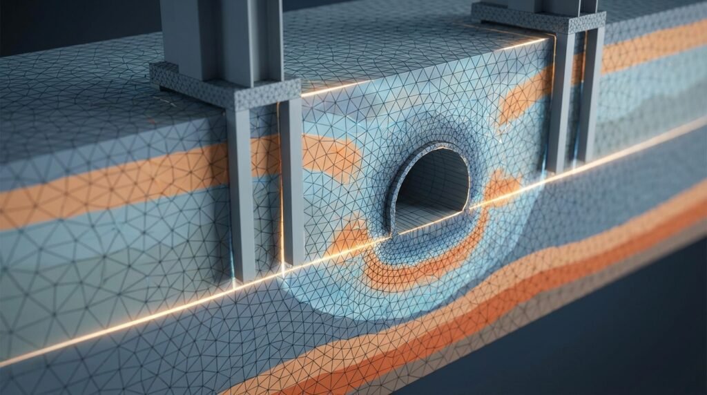
Soil modeling involves translating the complex mechanical behavior of soil into mathematical and computational frameworks. These models are then used in advanced analysis techniques, primarily Finite Element Analysis (FEA), to simulate real-world scenarios. From designing stable foundations for buildings and bridges to analyzing the integrity of pipelines in challenging terrains, a solid understanding of soil modeling is indispensable.

Illustrative image showing a finite element model of a strip foundation. Image courtesy of Wikimedia Commons.

Why Is Accurate Soil Modeling Critical in Engineering?

The implications of inaccurate soil modeling can range from costly design overruns to catastrophic structural failures. For engineers working across various disciplines, precision in simulating soil behavior is not just good practice—it’s a necessity.

Key Areas Benefiting from Robust Soil Modeling:

Structural Engineering & Foundations: Essential for designing foundations (shallow, deep, raft), retaining walls, and underground structures. Understanding soil-structure interaction is vital for predicting settlement, bearing capacity, and overall stability. This directly impacts the structural integrity of buildings and infrastructure.
Geotechnical Engineering: At its core, soil modeling underpins slope stability analysis, tunnel design, embankment construction, and landfill engineering. It helps predict ground movements, pore water pressure dissipation, and the potential for liquefaction.
Oil & Gas Industry: Critical for assessing pipeline integrity in unstable soil conditions, designing offshore platforms anchored to the seabed, and evaluating subsidence risks around extraction sites.
Aerospace & Infrastructure: While less direct than civil applications, soil modeling can be relevant for designing airport runways, taxiways, and specialized ground support equipment where soil interaction is a factor.
Forensic Engineering & Failure Analysis (FFS Level 3): When analyzing existing structures or investigating failures, advanced soil modeling can help recreate original conditions, assess degradation, and determine root causes. This is particularly relevant in Fitness-for-Service (FFS) assessments, especially Level 3, where complex non-linear analysis is often required.
Environmental Engineering: Used for analyzing contaminant transport through soil, designing liners for waste containment, and managing groundwater flow.

Without accurate soil models, designs can be overly conservative (leading to increased costs) or, worse, under-designed (leading to potential collapse or excessive deformations). It’s a balance of safety and economy.

Understanding Fundamental Soil Properties for Modeling

Before diving into constitutive models, it’s crucial to grasp the basic mechanical properties that define soil behavior. These parameters are the input data for any soil model.

Essential Soil Parameters:

Cohesion (c): Represents the shear strength of soil when there is no normal stress. Predominant in clays.
Angle of Internal Friction (φ): Represents the shear strength due to inter-particle friction. Predominant in sands and gravels.
Young’s Modulus (E) / Modulus of Elasticity: A measure of soil stiffness, indicating its resistance to elastic deformation under normal stress.
Poisson’s Ratio (ν): Describes the ratio of transverse strain to axial strain under uniaxial stress. For soils, it often ranges from 0.2 to 0.49.
Density (ρ): Mass per unit volume, critical for self-weight calculations.
Permeability (k): A measure of how easily water flows through the soil, crucial for consolidation and seepage analysis.
Compression Index (C_c) & Swelling Index (C_s): Parameters defining the compressibility and swelling characteristics of cohesive soils, particularly for consolidation analysis.
Shear Modulus (G): Related to Young’s Modulus and Poisson’s Ratio (G = E / (2(1+ν))), it describes the soil’s resistance to shear deformation.

These properties are typically determined through laboratory tests (e.g., triaxial compression, direct shear, oedometer) and in-situ field tests (e.g., Standard Penetration Test (SPT), Cone Penetration Test (CPT), pressuremeter tests).

Constitutive Models: The Heart of Soil Modeling

Constitutive models are mathematical relationships that describe the stress-strain behavior of materials. For soils, selecting the correct constitutive model is arguably the most critical step, as it dictates how the FEA software interprets the soil’s response to loading.

Common Constitutive Models for Soil:

Here’s a breakdown of commonly used models, from simplest to more complex:

Model Type	Description	Typical Application	Pros	Cons
Linear Elastic	Assumes ideal elastic behavior (stress proportional to strain) and isotropic properties. Simplest model.	Initial stress estimation, small strain analysis in very stiff soils, often a preliminary step.	Easy to implement, few parameters.	Doesn’t capture plasticity, strength limits, or non-linear behavior. Unrealistic for most soils.
Mohr-Coulomb	An elasto-plastic model based on a linear failure envelope. Widely used for frictional and cohesive soils.	Slope stability, retaining walls, shallow foundations. Good for many practical geotechnical problems.	Relatively simple, easy to understand parameters (c, φ).	Doesn’t account for strain hardening/softening, intermediate principal stress effects, or realistic volumetric changes. Corners in yield surface can cause numerical issues.
Drucker-Prager	Similar to Mohr-Coulomb but with a smoother, conical yield surface. Often used as an approximation of Mohr-Coulomb.	Problems requiring smooth yield surface for numerical stability, general geotechnical applications.	Smoother yield surface, better numerical convergence than Mohr-Coulomb in some cases.	Parameters need to be converted from Mohr-Coulomb. Similar limitations regarding strain hardening/softening.
Hardening Soil Model	An advanced elasto-plastic model that accounts for stress-dependent stiffness and isotropic hardening.	Embankments, deep excavations, tunneling, settlement analysis where stiffness variation with stress is important.	Captures stiffness non-linearity and permanent deformation more realistically than Mohr-Coulomb.	More parameters to determine, requires more advanced lab testing.
Modified Cam-Clay / Critical State Models	Based on critical state soil mechanics. Excellent for normally and over-consolidated clays. Accounts for volumetric changes during shearing.	Consolidation, settlement of clays, deep foundations in soft clays, tunneling.	Physically robust, captures contractive/dilative behavior and critical state.	Complex to understand and calibrate, requires specialized lab data. Primarily for cohesive soils.

Choosing the Right Model: A Practical Approach

Selecting the appropriate constitutive model involves a trade-off between accuracy, complexity, and available data. For many routine geotechnical designs, Mohr-Coulomb offers a good balance. For projects requiring high precision, such as large infrastructure or critical structures on soft soils, more advanced models like Hardening Soil or Modified Cam-Clay become necessary.

Key Takeaway: Always start with the simplest model that can reasonably represent the dominant behavior. Increase complexity only when justified by project requirements, available data, and the need for higher accuracy.

The FEA Workflow for Soil Modeling

Integrating soil models into a Finite Element Analysis (FEA) framework is the standard approach for simulating geotechnical problems. Here’s a typical workflow, emphasizing aspects specific to soil.

1. Geometry and Meshing:

Define Geometry: Model the soil domain, including all relevant layers, interfaces, and any embedded structures (e.g., foundations, piles). Consider the extent of the soil domain carefully; boundaries should be far enough from areas of interest to avoid artificial constraint effects.
Meshing: Generate an appropriate mesh. For soils, elements that can handle large deformations (e.g., quadratic elements, reduced integration elements) are often preferred. Finer meshes are needed in areas of high stress gradients, around structures, and near failure zones.

2. Material Property Assignment:

Layering: Assign different material properties (based on chosen constitutive models) to distinct soil layers identified from site investigations.
Parameter Input: Carefully input all derived soil parameters (c, φ, E, ν, permeability, etc.) into the FEA software. Double-check units and values.

3. Boundary Conditions (BCs) and Loading:

Displacement BCs: Typically, the bottom boundary of the soil domain is fixed in all directions. Vertical sides are usually constrained horizontally but allowed to move vertically, simulating free field conditions.
Pore Water Pressure BCs: For coupled consolidation or seepage analyses, define pore water pressure conditions (e.g., hydrostatic initial conditions, permeable/impermeable boundaries).
Loading: Apply structural loads (e.g., foundation pressure), hydrostatic pressures, seismic loads, or any other relevant forces. Apply loads incrementally if non-linear behavior is expected.

4. Analysis Type Selection:

Choose an analysis type that matches the problem:

Static Analysis: For immediate settlement, bearing capacity, and overall stability under static loads.
Consolidation Analysis: For time-dependent settlement due to pore water dissipation (especially in clays).
Dynamic Analysis: For seismic response, machine vibrations, or impact loads.
Coupled Flow-Deformation Analysis: For complex problems involving interaction between fluid flow (water) and soil deformation.

Relevant Software Tools for Soil Modeling

Modern FEA software packages offer robust capabilities for geotechnical modeling. Some of the industry leaders include:

Abaqus: A powerful general-purpose FEA tool with extensive material models, including various plasticity and critical state models for soils. Excellent for complex non-linear problems and highly customized simulations.
ANSYS Mechanical: Another versatile FEA suite offering specific geotechnical capabilities through its material models and element types. Good for soil-structure interaction.
PLAXIS: A specialized 2D and 3D FEA software designed specifically for geotechnical applications. It has a user-friendly interface for defining soil layers, constitutive models (including advanced ones like Hardening Soil, Soft Soil Creep), and common geotechnical analyses. Highly regarded in the geotechnical community.
GeoStudio (SLOPE/W, SIGMA/W, SEEP/W, etc.): A suite of integrated software for slope stability, deformation, seepage, and other geotechnical analyses. While some modules use limit equilibrium, SIGMA/W offers FEA capabilities for stress-deformation.
FLAC / FLAC3D: Explicit finite difference codes widely used for geotechnical and rock mechanics problems, especially those involving large deformations and material failure.
OpenFOAM: An open-source CFD tool, which with specialized solvers and libraries, can be adapted for some pore-fluid flow and consolidation problems, though it requires significant customization for solid mechanics of soils.

For CAD-CAE workflows, preliminary geometry might be created in tools like CATIA or AutoCAD, then imported into the FEA software for meshing and analysis.

Practical Workflow: A Step-by-Step Guide to Soil Modeling

Let’s walk through a practical example — say, analyzing the settlement of a shallow foundation on a layered soil profile.

Step 1: Data Gathering and Site Characterization

Obtain Geotechnical Report: This is your primary source of information. It should include bore logs, lab test results (triaxial, oedometer), field test data (SPT N-values, CPT qc/fs), and groundwater levels.
Define Soil Layers: Based on bore logs, identify distinct soil strata and their depths. For our foundation example, let’s assume a top layer of dense sand over a layer of normally consolidated clay.
Determine Material Properties: Extract or derive parameters (c, φ, E, ν, ρ, C_c, C_s, k) for each soil layer from the report. If values are ranges, choose representative values or perform sensitivity analysis.

Step 2: Model Setup in FEA Software (e.g., PLAXIS or Abaqus)

Create Geometry: Draw the soil domain (e.g., 2D plane strain or 3D model). Include the foundation geometry. Ensure the domain extends far enough laterally and vertically (e.g., 3-5 times foundation width, or until stiff layer is reached) to minimize boundary effects.
Assign Material Models:
- For the dense sand: A Mohr-Coulomb model is often sufficient for static settlement, or Hardening Soil if stiffness non-linearity is critical.
- For the normally consolidated clay: A Modified Cam-Clay or Hardening Soil Small Strain model would be appropriate for capturing consolidation and long-term settlement.
Input Material Parameters: Carefully input all derived c, φ, E, ν, density, and consolidation parameters for each assigned material model and layer.
Apply Boundary Conditions:
- Sides of the soil domain: restrained horizontally, free vertically.
- Bottom of the soil domain: restrained in all directions.
- For consolidation analysis, define permeable boundaries at the top and bottom of the clay layer if drainage is expected.
Apply Loading: Model the foundation load. This can be applied as a distributed pressure over the foundation area or as concentrated forces if modeling structural columns directly. Apply loads in stages if you are simulating construction sequences or if the soil exhibits strong non-linear behavior.

Step 3: Mesh Generation

Initial Mesh: Generate a coarse mesh for the entire domain.
Refine Mesh: Significantly refine the mesh around the foundation and within the soil layers directly affected by the load. Use finer elements where large deformations or stress concentrations are expected.

Step 4: Analysis Execution

Initial Stress State: Before applying any external loads, perform a ‘gravity loading’ or ‘initial stress’ step to establish the geostatic stress state in the soil due to its self-weight. This is crucial for accurate soil behavior.
Load Application Stages: Run the analysis, applying the foundation load incrementally. For consolidation, ensure the time stages are set appropriately to capture the pore pressure dissipation.

Step 5: Post-Processing and Interpretation

Review Deformations: Check the settlement profiles and total deformations. Is the settlement distribution reasonable? Are there any unexpected large displacements?
Examine Stresses and Strains: Analyze effective stresses, pore water pressures, and shear strains. Look for areas where the soil’s strength limits have been reached (yield zones).
Check Convergence: Ensure the solution has converged within acceptable tolerances. Non-convergence can indicate instability or incorrect model setup.
Compare with Hand Calculations/Empirical Methods: For simple cases, compare computed settlements with empirical methods (e.g., Terzaghi’s 1D consolidation theory, Schmertmann’s CPT method) as a sanity check.

Common Challenges and Troubleshooting in Soil Modeling

Soil modeling often presents unique challenges that require careful attention.

Material Parameter Calibration: One of the biggest hurdles. Lab test data can be scattered, and derived parameters for complex models may require significant engineering judgment or even specialized inverse analysis.
Convergence Issues: Highly non-linear soil behavior (e.g., plastic yielding, large deformations) can lead to difficulties in solution convergence. This often requires reducing load increments, adjusting solution controls, or refining the mesh.
Meshing for Large Deformations: When soil undergoes significant movement (e.g., slope failure, tunneling), traditional fixed meshes can become severely distorted, leading to element inversion or poor accuracy. Techniques like Arbitrary Lagrangian-Eulerian (ALE) formulation or remeshing algorithms might be necessary.
Defining Realistic Boundary Conditions: Incorrectly applying boundary conditions can over-constrain or under-constrain the soil domain, leading to inaccurate results.
Pore Water Pressure Effects: Neglecting the role of water (e.g., undrained vs. drained conditions, consolidation) can lead to fundamentally incorrect predictions, especially in fine-grained soils.

Troubleshooting Tips:

Start Simple: Begin with a simpler material model (e.g., linear elastic) to get a baseline and ensure geometry/BCs are correct before introducing complexity.
Check Deformations First: If convergence issues arise, check the deformation plots from the last converged increment. This often reveals localized instabilities.
Verify Material Properties: Ensure parameters are within expected ranges and units are consistent.
Iterative Refinement: Adjust load increments, mesh density, and solver settings incrementally.
Consult Documentation: Software manuals often have specific recommendations for geotechnical problems and common pitfalls.

Verification & Sanity Checks for Soil Simulations

Never trust a simulation blindly. Verification and validation are crucial.

Essential Checks:

Mesh Sensitivity Analysis: Run the simulation with different mesh densities. Your results (e.g., settlement, stress) should stabilize as the mesh gets finer, indicating mesh independence.
Boundary Condition Sensitivity: Slightly adjust the location of your domain boundaries. Do the results in the critical area change significantly? If so, your boundaries might be too close.
Comparison with Analytical Solutions: For simplified cases (e.g., settlement under a uniform load on an elastic half-space), compare your FEA results with classical analytical solutions.
Field Data and Empirical Methods: Where available, compare simulated results with actual field measurements (e.g., inclinometer readings, settlement plates) or established empirical correlations. This is the ultimate validation.
Energy Balance Checks: Most FEA software provides information on energy balance. Large imbalances can indicate numerical problems.
Visualization of Results: Visually inspect deformation patterns, stress contours, and failure zones. Do they make physical sense? Are stress bulbs distributed as expected?

For complex projects or when introducing new material models, consider seeking expert review or leveraging external consulting services. EngineeringDownloads.com offers specialized online consultancy and tutoring to help you navigate these advanced challenges effectively.

Leveraging Python & MATLAB for Geotechnical Automation

Python and MATLAB are invaluable tools for enhancing your soil modeling workflow, especially in CAD-CAE integration and automation.

Parametric Studies: Automate running multiple FEA simulations with varying soil parameters (e.g., friction angle, modulus), foundation sizes, or load magnitudes. This helps in understanding design sensitivities and optimizing designs.
Pre-processing: Generate complex 3D soil geometries, define layered stratigraphy, and automatically assign material properties using scripts. This is particularly useful for models with many layers or irregular interfaces.
Post-processing & Data Extraction: Extract specific results (e.g., maximum settlement, pore pressures at specific locations, stress paths) from large FEA output files. Python libraries like NumPy and SciPy, and MATLAB’s robust data handling, are excellent for this.
Calibration & Inverse Analysis: Develop scripts to iteratively adjust soil model parameters to match laboratory or field test data more closely. This can significantly improve the accuracy of your models.
Visualization: Create custom plots and visualizations of FEA results, perhaps combining them with site investigation data for a more comprehensive understanding.
Integration: Many commercial FEA packages (Abaqus, ANSYS) offer Python APIs, allowing direct interaction with the software for model building, analysis submission, and result extraction.

Explore EngineeringDownloads.com for downloadable Python and MATLAB scripts designed for geotechnical data analysis and FEA workflow automation.

Future Trends in Soil Modeling

The field of soil modeling continues to evolve rapidly. Expect to see:

Increased Use of Machine Learning (ML): ML algorithms are being explored for material parameter calibration, predicting soil behavior from limited data, and even accelerating complex simulations.
Advanced Constitutive Models: Development of more sophisticated models that better capture anisotropy, time-dependent behavior (creep), cyclic loading effects (liquefaction), and thermo-hydro-mechanical coupling.
Digital Twins: Creation of virtual replicas of geotechnical assets that integrate real-time sensor data with predictive soil models for continuous monitoring and maintenance.
High-Performance Computing (HPC): Leveraging cloud computing and parallel processing to run increasingly complex and large-scale geotechnical simulations more efficiently.

Conclusion: Mastering the Ground Beneath Our Feet

Soil modeling is an intricate but indispensable aspect of modern engineering. By carefully selecting constitutive models, diligently characterizing soil properties, and meticulously setting up and verifying FEA simulations, engineers can confidently design structures that stand the test of time and environmental challenges. It’s a journey of continuous learning and refinement, where practical application meets theoretical understanding.

Embrace the complexity, leverage the tools available, and remember that a well-modeled soil foundation is the bedrock of any successful engineering project.