Pressure Outlet Backflow in CFD: A Practical Engineering Guide

CFD
Engineering Downlaods
March 23, 2026
18 Minute

In the world of Computational Fluid Dynamics (CFD), achieving accurate and stable simulations is paramount. One common challenge that can lead to significant headaches and erroneous results is pressure outlet backflow. This phenomenon occurs when fluid flows back into the computational domain through a designated pressure outlet boundary condition, defying the intended outward flow.

Understanding, identifying, and effectively mitigating pressure outlet backflow is a critical skill for any engineer working with CFD, whether you’re simulating complex turbomachinery, analyzing flow in an oil & gas pipeline, or designing a biomedical device. This guide will walk you through the intricacies of backflow, offering practical insights and actionable strategies to ensure your simulations are robust and reliable.

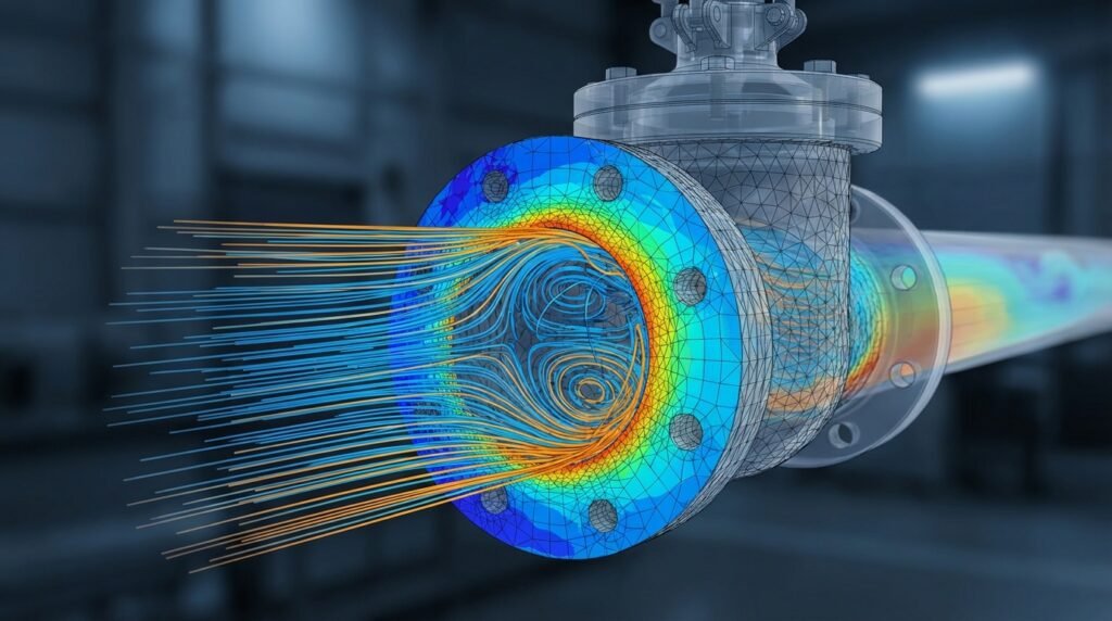
Illustrative CFD visualization of fluid streamlines around a wind turbine, demonstrating complex flow patterns within a computational domain.

Understanding Pressure Outlet Backflow

Pressure outlets are fundamental boundary conditions in CFD, designed to allow fluid to exit the computational domain where the pressure is known or can be estimated. However, these conditions aren’t always straightforward.

The Nature of Pressure Outlets in CFD

A pressure outlet boundary condition typically extrapolates flow variables (like velocity components and temperature) from the interior of the domain to the boundary face. It allows fluid to exit the domain freely, and if the flow tries to enter the domain (backflow), the solver often assigns inlet-like conditions (e.g., zero normal gradient for velocity components, specified turbulence quantities, or even fixed total temperature).

How they work: The solver determines the local mass flow rate based on the specified static pressure at the outlet and the flow conditions approaching it.
When backflow typically occurs: Backflow arises when the pressure inside the domain, near the outlet, is significantly lower than the specified pressure at the outlet boundary, or when an adverse pressure gradient causes flow separation and recirculation zones that extend to or across the outlet. This can happen due to:
- Poorly designed geometry (sharp turns, sudden expansions).
- Under-resolved flow features near the outlet.
- Incorrectly specified outlet pressure.
- Unsteady phenomena pushing flow upstream.

Why Backflow Matters: Impact on Your Simulation

Pressure outlet backflow is not just a warning message; it’s a symptom of a deeper problem that can invalidate your entire simulation. Its impact is far-reaching:

Convergence issues: Backflow is a primary culprit for solver divergence, oscillations, or extremely slow convergence. The solver struggles to maintain stability when inflow conditions are imposed where outflow is expected.
Inaccurate results: Even if your simulation appears to converge, backflow can lead to physically unrealistic results. Mass conservation might be violated, flow profiles could be distorted, and critical parameters like drag, lift, or heat transfer coefficients will be incorrect. In structural engineering contexts, incorrect fluid forces from an inaccurate CFD could lead to miscalculated stresses in a subsequent Fluid-Structure Interaction (FSI) analysis using tools like Abaqus or ANSYS Mechanical.
Physical interpretation challenges: It becomes difficult to trust any results near the outlet, complicating design decisions and performance evaluations.

Identifying Pressure Outlet Backflow in Your Simulation

Before you can fix backflow, you need to know it’s happening. Modern CFD software like ANSYS Fluent, ANSYS CFX, and OpenFOAM provide clear indicators.

Solver Messages and Warnings

Keep a close eye on your solver console or log file. You’ll often see explicit warnings:

'Reversed flow at pressure outlet X on X faces' (ANSYS Fluent)
'CFX Warning: Reverse flow occurred at an Outlet boundary' (ANSYS CFX)
Similar messages in OpenFOAM indicating negative flux or cells with reverse flow.
Significant fluctuations or non-zero residuals for continuity and velocity components.

Don’t ignore these warnings, even if the simulation seems to progress.

Post-Processing Visualizations

Visual inspection in post-processors like CFD-Post, ParaView, or custom Python/MATLAB scripts is crucial:

Velocity vectors: Plotting velocity vectors on the outlet plane or a plane just upstream will immediately reveal any vectors pointing inward.
Streamlines/Pathlines: Release streamlines from points near the outlet. If they curl back into the domain, you have backflow.
Pressure contours: Inspect pressure contours near the outlet. An unexpectedly low pressure region immediately upstream of the outlet can indicate a potential for backflow.
Mass flow rate monitoring: Monitor the mass flow rate at all inlets and outlets. A negative mass flow at a pressure outlet (where positive is outward) is a definitive sign of backflow. This can be easily scripted using Python for automated checks.
Iso-surfaces: Create an iso-surface of the velocity component normal to the outlet plane where its value is negative. This will highlight precisely where and how much backflow is occurring.

Practical Workflow: Preventing and Mitigating Backflow

Addressing pressure outlet backflow often requires a multi-pronged approach, focusing on geometry, mesh, and solver settings.

Mesh Design Strategies

Mesh quality and domain extent play a significant role in preventing backflow.

Extending the outlet domain: This is arguably the most effective strategy. Extend the physical domain downstream by 5 to 10 hydraulic diameters (or characteristic lengths). This allows the flow to fully develop and become nearly uniform before it exits, minimizing the chance of recirculation zones impinging on the boundary.
Refining the mesh near the outlet: A sufficiently fine and structured mesh at the outlet can help the solver accurately resolve gradients and reduce numerical errors that might contribute to backflow.
Orthogonality: Ensure the mesh cells at the outlet plane are highly orthogonal to the boundary. Poor orthogonality can lead to interpolation errors.
Boundary layer considerations: If there are walls extending to the outlet, ensure proper boundary layer meshing (e.g., appropriate y+ values) to accurately capture near-wall physics that might influence the overall flow direction.

Boundary Condition Setup (Crucial!)

The choice and specification of boundary conditions are paramount.

Choosing the right outlet BC:
- Pressure Outlet: The standard choice, where static pressure is specified. Be careful with its value.
- Outflow: Less common in industrial CFD, it assumes fully developed flow and zero diffusion fluxes. It can be less stable than a pressure outlet if backflow occurs.
- Pressure Far-Field: Used for external aerodynamics, where the boundary is far from the object. It treats the boundary as an acoustic non-reflecting boundary.
- Total Pressure Outlet: If you know the total pressure at the outlet, this can be more robust as it sets a more definite condition.
Specifying gauge vs. absolute pressure: Always be clear whether your specified pressure is gauge or absolute. In most CFD tools like Fluent, the default operating pressure is 1 atm, and specified pressures are gauge relative to this. Misinterpreting this can cause large, unphysical pressure differences leading to backflow.
Avoiding overly restrictive conditions: Don’t try to force an outlet where the physics dictates inflow or strong recirculation. Let the flow develop naturally.
Flow Split Ratio (Fluent): If you have multiple outlets, you can sometimes use a flow split ratio, but this is less common for preventing backflow directly.

Solver Settings and Stabilization Techniques

Even with good mesh and BCs, solver settings can help stabilize a tricky case.

Under-relaxation factors: Gradually reduce under-relaxation factors for pressure and momentum. This slows down the solution update, making it more stable, though it increases solution time.
Solution initialization strategies: Initialize the flow field with reasonable values, perhaps from a simpler, coarser mesh run, or a potential flow solution. Avoid ‘patching’ unrealistic values near the outlet.
Double precision: Always use double precision for complex or sensitive simulations to minimize numerical errors.
Pressure-velocity coupling schemes: Algorithms like SIMPLE, PISO, or COUPLED (Fluent/CFX) have different strengths. COUPLED is often more robust but computationally intensive. Experiment if stability is an issue.
Transient vs. Steady-state considerations: If the flow is inherently unsteady, a steady-state simulation might struggle to converge or show persistent backflow. Switching to a transient (unsteady) simulation can reveal the true flow physics and resolve the backflow issue, as it allows the flow features to evolve over time.

Geometric Modifications

Sometimes, the root cause is the physical design itself.

Diffuser design: If the outlet is part of a diffuser, ensure the divergence angle is not too steep, as this can cause flow separation and backflow.
Smoothing sharp turns: Aggressive changes in flow direction can create recirculation. Radius sharp corners or introduce guide vanes if physically plausible.
Flow straighteners: In some experimental setups, flow straighteners are used upstream of outlets to ensure uniform flow. While not always practical for simulation geometry, it highlights the ideal flow condition.

Here’s a quick summary of common backflow scenarios and typical solutions:

Scenario	Primary Cause	Recommended Solutions	Tools (Examples)
Recirculation at outlet	Short domain, adverse pressure gradient, sharp geometry	Extend domain, smooth geometry, refine outlet mesh	Fluent, CFX, OpenFOAM (Meshing tools like ICEM CFD, snappyHexMesh)
Solver divergence	Unstable conditions, unphysical BC, large time step (transient)	Adjust under-relaxation, improve initialization, use smaller time step	Fluent, CFX, OpenFOAM (Solver settings)
Low interior pressure	Overly high specified outlet pressure, incorrect gauge/absolute reference	Verify outlet pressure value, check operating pressure, switch to mass flow outlet if known	Fluent, CFX (Boundary Condition panel)
Unsteady flow impacting outlet	Turbulence, vortex shedding near outlet	Switch to transient simulation, extend domain significantly	Fluent (Transient solver), CFX (Transient run), OpenFOAM (PIMPLE algorithm)

Verification & Sanity Checks for Robustness

Even after addressing backflow, several checks are essential to ensure the reliability of your CFD results.

Grid Independence Study

Perform simulations on at least three different mesh resolutions (coarse, medium, fine). If key output parameters (e.g., mass flow rate, pressure drop, velocity profile) change significantly with mesh refinement, your results are mesh-dependent. Ensure your final mesh produces grid-independent results, especially at the outlet.

Sensitivity Analysis

Test the sensitivity of your results to small variations in boundary conditions (e.g., a ±5% change in outlet pressure) or turbulence model parameters. This helps confirm that your solution is not overly sensitive to minor input fluctuations and reflects physical reality. For instance, comparing k-epsilon with k-omega SST can reveal model dependency.

Mass Flow Balance Check

For any incompressible, steady-state simulation, the total mass flow rate entering the domain must equal the total mass flow rate exiting. For compressible flows, this applies to steady state. For transient compressible flows, the net mass accumulation in the domain should equal the net mass flow across boundaries. Always verify this. A significant imbalance (e.g., > 0.1% of total flow) often indicates a problem, potentially unresolved backflow or poor convergence.

Physical Plausibility Check

Do your results make sense? Are the velocity profiles reasonable? Are pressure gradients consistent with expected flow behavior? Compare with analytical solutions, empirical correlations, or experimental data if available. This crucial sanity check helps catch fundamental errors.

Monitoring Wall Y+

If your geometry includes walls, ensure your y+ values are within the appropriate range for your chosen turbulence model (e.g., y+ ~ 1 for low-Reynolds number models or y+ > 30 for wall functions). Incorrect y+ can lead to inaccuracies that affect the entire flow field, potentially contributing to unexpected flow behavior near outlets.

Advanced Troubleshooting for Persistent Backflow

When basic strategies aren’t enough, consider these advanced techniques.

Adjusting Turbulence Models

Some turbulence models are more prone to predicting flow separation or recirculation than others. For example, the k-epsilon model can sometimes overpredict turbulence in adverse pressure gradient regions. Switching to a more advanced model like k-omega SST, which is known for better performance in separated flows and near-wall regions, might improve stability and prevent backflow.

Utilizing Source Terms (with caution)

In rare, highly specialized cases, you might introduce a small momentum source term near the outlet to gently push flow outward. This is generally a last resort and should be used with extreme caution, as it artificially alters the flow and can compromise the physical accuracy of your simulation. It’s more of a numerical stabilization trick than a physical solution.

Adaptive Meshing

For highly complex and evolving flow fields, adaptive meshing (dynamic mesh refinement) can be invaluable. It refines the mesh in regions of high gradients or where specific flow features (like vortices causing backflow) are detected. This ensures that critical areas, including potential backflow zones, are adequately resolved without over-meshing the entire domain.

Transient Simulations for Unsteady Phenomena

If your steady-state simulation consistently shows backflow, the underlying physics might be inherently unsteady. Transient simulations can capture the temporal evolution of flow features, such as vortex shedding or pulsatile flow, which a steady-state solver cannot. This often resolves backflow warnings as the solver can follow the natural oscillations of the flow rather than trying to force an artificial steady state.

Real-World Implications and Case Studies (Illustrative)

The lessons learned from managing pressure outlet backflow apply across many engineering disciplines.

Oil & Gas Pipelines

Simulating flow through valves, pumps, and pipe junctions often involves complex recirculation. If an outlet is placed too close to a valve or a bend, backflow warnings are common. Ensuring sufficient pipe length downstream of such components in the CFD model is critical for accurate pressure drop and flow distribution predictions.

Aerospace Components (Nozzles, Inlets)

Accurate prediction of flow through jet engine nozzles or air intakes is vital. Backflow at a nozzle exit, for instance, could indicate an improperly modeled expansion or over-expansion, leading to incorrect thrust calculations. Inlets at high angles of attack might experience significant flow separation, leading to backflow at a downstream boundary if the domain is too short.

Biomechanics (Blood Flow in Arteries)

When modeling blood flow through arteries, especially with stents or aneurysms, localized recirculation zones are common. If an ‘outlet’ in the computational model is placed within such a zone or too close to it, backflow can occur, invalidating Wall Shear Stress (WSS) and residence time calculations, which are crucial for predicting disease progression. Biomechanics simulations in tools like Fluent or OpenFOAM heavily rely on accurate boundary conditions.

CAD-CAE Workflows: Integrating CFD Findings

Addressing backflow isn’t just a CFD problem; it’s a design problem. When CFD identifies persistent backflow due to geometry, this feeds back into the CAD stage (e.g., using CATIA or SolidWorks) for design modification. The improved geometry then undergoes re-analysis, highlighting the iterative nature of CAD-CAE workflows.

Leveraging Python & MATLAB for Backflow Analysis

Beyond the standard CFD software interfaces, scripting languages offer powerful capabilities for diagnosing and reporting backflow.

Automated Post-Processing Scripts

You can write Python or MATLAB scripts to:

Monitor mass flow rates: Automatically extract and plot mass flow rates at all outlets over time or iteration, quickly highlighting any negative values.
Identify regions of backflow: Extract velocity data from the outlet plane and calculate the normal component. Script to identify and quantify the area or percentage of the outlet experiencing negative normal velocity.
Plot critical parameters: Generate custom plots of pressure, velocity, or turbulence quantities at specified locations or lines near the outlet for detailed inspection.

These scripts integrate seamlessly with popular CFD packages, allowing for efficient, reproducible analysis. For instance, Fluent has a TUI (Text User Interface) that can be driven by Python, and OpenFOAM uses native Python scripting for post-processing with libraries like PyFoam or general plotting libraries.

Data Extraction and Reporting

Automate the generation of summary reports including backflow statistics, convergence history, and mass balance checks. This is invaluable for large projects or parametric studies, helping you quickly identify problematic simulations and focus on troubleshooting.

Enhance Your CFD Skills with EngineeringDownloads.com

Mastering complex CFD phenomena like pressure outlet backflow requires continuous learning and practical application. EngineeringDownloads.com offers a wealth of resources to help you sharpen your skills. Explore our collection of downloadable CFD project templates, Python and MATLAB scripts for advanced post-processing and automation, or connect with our experienced engineers for one-on-one online consultancy and tutoring services to tackle your most challenging simulation problems.

Conclusion: Master Your CFD Outlets

Pressure outlet backflow is a pervasive issue in CFD, but it’s one that can be effectively managed with a systematic approach. By carefully considering your computational domain’s extent, refining your mesh, selecting appropriate boundary conditions, and understanding your solver’s capabilities, you can achieve stable, accurate, and physically plausible results. Embracing advanced troubleshooting and leveraging powerful scripting tools will further solidify your expertise, ensuring you can confidently navigate even the most challenging fluid dynamics simulations.