FEA Principles: A Practical Guide for Modern Engineers

Demystifying FEA Principles: Your Practical Engineering Handbook

Finite Element Analysis (FEA) is an indispensable tool in modern engineering, transforming how we design, analyze, and validate structures and components. From ensuring the structural integrity of an aerospace wing to optimizing biomechanical implants, FEA allows engineers to predict real-world behavior under various loads and conditions without costly physical prototypes.

But what exactly underpins this powerful simulation method? This guide will break down the fundamental FEA principles, offer practical workflow advice, highlight common pitfalls, and equip you with the knowledge to perform reliable and accurate simulations. Whether you’re working with Abaqus, ANSYS Mechanical, or exploring open-source alternatives, understanding these core concepts is your first step to mastering the art of numerical simulation.

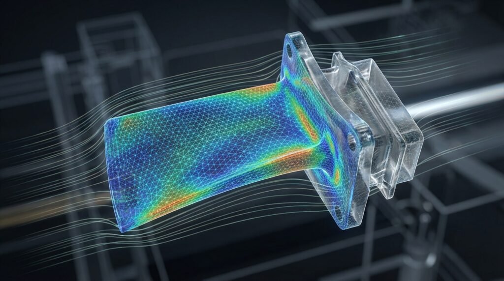
A visual representation of a beam discretized into finite elements for FEA.

What is Finite Element Analysis (FEA)?

At its heart, FEA is a numerical method for solving complex engineering problems involving differential equations. Instead of trying to solve the problem across the entire continuous domain (which is often impossible analytically), FEA breaks down a complex structure into many smaller, simpler parts called ‘finite elements’. These elements are interconnected at ‘nodes’.

By approximating the behavior within each simple element and then assembling these approximations for the entire structure, FEA can provide highly accurate predictions of stress, strain, deformation, heat transfer, fluid flow, and more. It’s the backbone of CAE (Computer-Aided Engineering) and crucial for FFS Level 3 assessments in oil & gas, among many other applications.

The Core Principles of FEA Explained

Understanding these foundational concepts is key to building effective and trustworthy FEA models.

Discretization: The Art of Meshing

The first and arguably most critical step in FEA is discretization, commonly known as meshing. This involves dividing your continuous physical domain (your component or structure) into a finite number of smaller, geometrically simpler regions called elements.

Elements: These are the building blocks of your FEA model. Common types include 1D beams/trusses, 2D shells/plates, and 3D solids (tetrahedrons, hexahedrons). The choice of element type significantly impacts accuracy and computational cost.
Nodes: These are the points where elements connect. Nodes hold the primary solution variables (e.g., displacements, temperatures, pressures) known as Degrees of Freedom (DOFs). Each node typically has 1 to 6 DOFs, depending on the element type and analysis dimensionality.

The quality, size, and type of elements in your mesh directly influence the accuracy and convergence of your solution. A finer mesh (smaller elements) generally leads to more accurate results but increases computational time.

Material Models: Defining Reality

Every engineering material behaves differently under load. FEA requires you to define these behaviors through material models. The complexity of the model depends on the material and the expected loading conditions.

Linear Elastic Isotropic: The simplest and most common model. It assumes a linear relationship between stress and strain (Hooke’s Law) and that properties are uniform in all directions. Defined by Young’s Modulus (E) and Poisson’s Ratio (ν).
Non-linear Material Models: For situations involving large deformations or stresses beyond the yield point, non-linear models are essential. These include:
- Plasticity: For metals exceeding their elastic limit.
- Hyperelasticity: For rubber-like materials (e.g., elastomers in biomechanics).
- Creep/Viscoelasticity: For materials under sustained load over time or temperature.
Anisotropic/Orthotropic: Materials whose properties vary with direction (e.g., composites, wood).

Boundary Conditions (BCs) and Loads: Simulating the Environment

Boundary conditions and loads represent how your component interacts with its surroundings. They dictate how the structure is constrained and what forces or environmental effects it experiences.

Boundary Conditions (Constraints): These restrict the motion (displacements or rotations) of specific nodes or surfaces. Common types include:
- Fixed (Encastre): All DOFs are constrained (e.g., a wall connection).
- Pinned: Translational DOFs are constrained, but rotational DOFs are free.
- Roller: Constraints only in the normal direction, allowing tangential movement.
- Symmetry: Used to model a portion of a symmetric structure, reducing model size.
Loads: These are the external forces, pressures, or environmental effects applied to your model.
- Concentrated Forces: Applied at specific nodes.
- Distributed Loads/Pressure: Applied over surfaces or edges.
- Body Forces: Act throughout the volume (e.g., gravity, centrifugal force).
- Thermal Loads: Temperature changes causing thermal expansion/contraction.
- Prescribed Displacements: Applying a known displacement rather than a force.

Formulating the Governing Equations

Once you’ve defined your elements, materials, BCs, and loads, the FEA software mathematically formulations a system of algebraic equations for the entire structure. For static structural analysis, this typically takes the form of: [K]{U} = {F}

[K] (Stiffness Matrix): Represents the stiffness of the entire structure, assembled from the individual element stiffness matrices.
{U} (Displacement Vector): The unknown nodal displacements that the solver aims to find.
{F} (Force Vector): The vector of applied nodal forces and reactions.

For more complex analyses (e.g., dynamic, non-linear), the equations become more involved, often requiring iterative solution methods.

Solving and Post-Processing

The solver in your FEA software (e.g., Abaqus/Standard, ANSYS Mechanical’s built-in solver) computes the unknown nodal displacements by solving the system of equations. Once displacements are known, elemental strains and stresses can be calculated. Post-processing involves visualizing and interpreting these results.

The FEA Workflow: A Practical Step-by-Step Guide

A structured approach to FEA ensures robust and reliable simulations. This practical workflow is applicable across various CAD-CAE tools like CATIA with its Generative Structural Analysis module, Abaqus, and ANSYS Mechanical.

1. Problem Definition and Scope

Clearly define what you need to achieve. What are the objectives? What specific results are you looking for (stress, deformation, natural frequency, etc.)? What assumptions are you making? What safety factors are relevant?

2. Geometry Preparation

Start with your CAD model. Simplify the geometry by removing small features (fillets, chamfers, small holes) that won’t significantly affect the overall structural behavior but would complicate meshing and increase computational cost. This is crucial for efficient CAE workflows.

3. Meshing Strategy

Choose appropriate element types (e.g., solid for bulky parts, shells for thin-walled structures, beams for slender members). Determine global mesh size and local refinements in areas of high stress gradients, load application, or boundary conditions. Aim for a balanced mesh quality.

4. Material Properties Assignment

Accurately input material properties (Young’s Modulus, Poisson’s Ratio, Yield Strength, Density, Thermal Expansion Coefficient, etc.) into the model. Ensure units consistency!

5. Boundary Conditions and Loading Application

Apply realistic constraints and loads that mimic the real-world operational environment. Pay extreme attention to this step, as incorrect BCs are a leading cause of inaccurate results. Consider gravity, temperature effects, and contact interactions.

6. Solver Setup and Execution

Select the appropriate analysis type (static, dynamic, thermal, non-linear, buckling). Configure solver parameters (e.g., time steps for transient analysis, number of iterations for non-linear). Run the simulation. For large models, this might be where Python or MATLAB scripting can automate batch runs or parameter studies.

7. Post-Processing and Interpretation

Visualize results (stress contours, displacement plots). Critically analyze the data. Do the results make sense physically? Are maximum stresses in expected areas? Is deformation realistic? Use stress linearization for pressure vessel assessments, for instance, or fracture mechanics parameters for FFS Level 3.

Key Considerations & Best Practices

Meshing Quality is Paramount

Poor mesh quality can lead to inaccurate results or even solver divergence. Key metrics to monitor include:

Aspect Ratio: Ratio of longest edge to shortest edge. Ideally close to 1:1, especially for 3D solids. High aspect ratios can cause numerical inaccuracies.
Skewness: Deviation of an element from its ideal shape (e.g., equilateral triangle, square). High skewness reduces accuracy.
Jacobian Ratio: Measures the distortion of an element. Large Jacobian values indicate severe distortion.
Warpage: For shell elements, how much the element deviates from a planar surface.

Modern pre-processors in tools like MSC Patran or Abaqus/CAE provide robust mesh quality checks.

Achieving Convergence

Convergence ensures that your solution is independent of further mesh refinement or increases in element order.

h-convergence (Mesh Refinement): Systematically refine the mesh (reduce element size) and observe how key results (e.g., maximum stress, deflection) change. When results stabilize, you’ve likely converged.
p-convergence (Element Order): Increase the polynomial order of the interpolation functions within elements (e.g., from linear to quadratic elements) while keeping the mesh geometry fixed. This often leads to faster convergence for smooth solutions.

Addressing Non-linearities

Many real-world problems are non-linear, requiring iterative solutions and careful setup.

Geometric Non-linearity: Occurs when deformations are large enough to significantly change the stiffness of the structure (e.g., buckling, snap-through).
Material Non-linearity: Material properties change with stress, strain, or temperature (e.g., plasticity, hyperelasticity).
Contact Non-linearity: Surfaces come into contact or separate during loading, altering load paths and constraints. This is common in assemblies and critical for many structural integrity assessments.

Units Consistency: A Silent Killer

Always maintain a consistent unit system throughout your model (geometry, materials, loads, BCs). A mix of inches, millimeters, pounds, and newtons is a recipe for disaster. Tools like ANSYS often have unit systems built-in, but user vigilance is key.

Computational Cost vs. Accuracy Trade-off

Finer meshes, complex material models, and non-linear analyses significantly increase computational time and resources. Balance the need for accuracy with practical project deadlines and available computing power. Sometimes, a simpler model can provide sufficient insight for preliminary design stages.

Practical Workflow: Stress Analysis of a Bracket

Let’s consider a practical example: analyzing a simple bracket fixed at one end with a load applied at the other. This scenario highlights a typical CAD-CAE workflow.

CAD Model: Start with the bracket’s geometry in CATIA, SolidWorks, or similar CAD software.
Import & Simplify: Import into your FEA pre-processor (e.g., Abaqus/CAE, ANSYS Mechanical interface). Remove small holes or fillets if they aren’t critical to the stress concentration areas you’re focusing on.
Material Properties: Assign an appropriate material, say structural steel, with its Young’s Modulus and Poisson’s Ratio.
Meshing: Generate a solid mesh (e.g., hexahedral elements if geometry permits, otherwise tetrahedral). Refine the mesh near the fixed end and the load application point, as these are expected stress concentration zones.
Boundary Conditions: Apply ‘Fixed’ constraints (zero displacement and rotation) to the bolt holes or the surface where the bracket is mounted.
Loading: Apply a force or pressure load to the area where the bracket supports a component.
Analysis Type: Select ‘Static Structural’ analysis.
Solve: Run the simulation.
Post-processing: Review stress (e.g., von Mises stress) contours to identify peak stress locations and compare them against the material’s yield strength. Check displacements for overall stiffness.

For repetitive tasks like varying the load or material, scripting in Python (e.g., with Abaqus Scripting Interface, or PyMAPDL for ANSYS) or MATLAB can automate the process, generating multiple simulation runs and extracting key data efficiently.

Verification & Sanity Checks: Trust but Verify

Never blindly trust FEA results. Always perform rigorous checks.

Analytical/Hand Calculations: For simplified versions of your problem (e.g., a simple beam bending for a complex structure), compare FEA results with classical engineering formulas. This is a crucial sanity check for overall deflection and global stress.
Symmetry Checks: If your model is symmetric, ensure that results (displacements, stresses) are symmetric. Deviations indicate incorrect BCs or model setup errors.
Reaction Forces: Sum the reaction forces at your constraints. They should ideally balance the applied loads. This is a fundamental equilibrium check.
Deformation Pattern: Does the deformation make physical sense? Is the part deflecting in the expected direction under the applied loads? If your model ‘blows up’ or deforms erratically, it often points to unconstrained rigid body motion (missing BCs).
Mesh Sensitivity Study: As discussed under convergence, perform this systematically. Results should stabilize as the mesh is refined.
Sensitivity to Boundary Conditions: Slightly perturb your boundary conditions (e.g., change a fixed support to a pin support in a less critical area) and observe the impact. This helps understand the model’s robustness.
Comparison with Experimental Data: The ultimate validation. If experimental data is available from lab tests, compare your FEA predictions directly. This builds confidence in your modeling approach for future similar problems.
Physical Interpretation: Always step back and ask: ‘Is this physically possible?’ Extreme stresses at a single node, oscillations in static results, or deflections orders of magnitude off are red flags.

Common Mistakes in FEA and How to Avoid Them

Incorrect or Insufficient Boundary Conditions: The most common error. Forgetting to constrain a DOF can lead to rigid body motion and solver divergence. Always check reaction forces and deformation plots.
Poor Mesh Quality: Using coarse or highly distorted elements in critical regions leads to inaccurate stress predictions. Invest time in mesh refinement and quality checks.
Ignoring Non-linearities: Assuming linear behavior for problems involving large deformations, plasticity, or contact can lead to grossly underestimated or overestimated stresses.
Material Property Errors: Incorrect input values (e.g., using MPa instead of GPa for Young’s Modulus) can yield results orders of magnitude off. Double-check all inputs.
Misinterpreting Results: Stresses are often singular at sharp corners in theoretical models. Don’t take peak stresses at these singularities as gospel for failure prediction. Focus on stresses away from singularities or use fatigue assessment methods.
Over-reliance on ‘Pretty Pictures’: Color contour plots are great for visualization but can hide inaccuracies. Always inspect numerical values, run sensitivity studies, and perform sanity checks.

Troubleshooting Common FEA Issues

Solver Divergence

When the solver fails to converge on a solution, especially in non-linear analyses, it often indicates a fundamental problem.

Check for Rigid Body Motion: Ensure all DOFs are adequately constrained. Look for warning messages about large rotations or displacements.
Review Material Properties: Are they realistic? Is the material model appropriate for the loading?
Check Load Steps/Increments: For non-linear analyses, smaller load increments can help convergence.
Contact Issues: Unstable contact definitions can cause divergence. Ensure contact is well-defined and initiated.

Excessive or Unrealistic Deformation

If your part deforms far beyond physical expectation:

Unit Consistency: Re-check all units.
Material Properties: Is Young’s Modulus too low? Is Poisson’s ratio correct?
Load Magnitude: Have you accidentally applied a load that is orders of magnitude too high?
Boundary Conditions: Are there sufficient constraints?

Unexpected Stress Concentrations

Stresses are high in areas you didn’t anticipate:

Load Path: Trace the load path through the structure. Are there sudden changes in stiffness or geometry?
Local BCs: Are your local boundary conditions accurate? For example, concentrated forces applied to a single node can cause artificial stress singularities.
Mesh Refinement: Ensure adequate mesh refinement in these areas to capture the stress gradient accurately.

The Role of Software and Automation

Modern FEA software packages like Abaqus, ANSYS Mechanical, and MSC Nastran/Patran offer comprehensive tools for pre-processing, solving, and post-processing. They handle complex geometries, advanced material models, and various analysis types with robust solvers.

For specialized applications, OpenFOAM, primarily a CFD tool, can be used for fluid-structure interaction (FSI) or coupled-field problems, requiring different meshing strategies and solvers.

Automation is increasingly vital in advanced CAE workflows. Python scripting, often integrated directly into commercial software (e.g., Abaqus Scripting Interface, ANSYS PyMAPDL), allows engineers to:

Automate repetitive pre-processing tasks (geometry modification, meshing).
Run parametric studies (varying dimensions, materials, loads).
Extract and process results efficiently from multiple simulations.
Integrate FEA with optimization algorithms.

MATLAB also plays a significant role in developing custom FEA solvers, post-processing utilities, and integrating with other analysis tools, especially in research and academic settings, or for specific control system interactions.

For those looking to deepen their expertise, EngineeringDownloads.com offers downloadable templates, scripts, and project files to kickstart your FEA automation journey, alongside expert tutoring and online consultancy services for complex simulation challenges.

Conclusion

Mastering FEA principles is an ongoing journey of learning and critical thinking. It empowers engineers to push boundaries, innovate, and ensure the safety and performance of critical components across industries like oil & gas, aerospace, and biomechanics. By understanding the core concepts, meticulously following workflows, and rigorously verifying your results, you’ll harness the true power of Finite Element Analysis and become a more effective and confident engineer.

Frequently Asked Questions About FEA Principles

FEA Element Type	Description	Typical Application
1D (Beam/Truss)	Models slender structures where cross-section deformation is negligible. Nodes have translational and rotational DOFs (beams) or only translational (trusses).	Frames, bridges, lattice structures, pipelines (global analysis).
2D (Shell/Plate)	Models thin-walled structures where one dimension is significantly smaller than the other two. Nodes have translational and rotational DOFs.	Sheet metal parts, aircraft skins, pressure vessel walls, automotive body panels.
3D (Solid/Brick/Tet)	Models bulky structures where all three dimensions are comparable. Nodes have translational DOFs only. Captures through-thickness stresses.	Engine blocks, complex castings, solid components, thick brackets, biomechanical implants.