Computational Fluid Dynamics (CFD) is an incredibly powerful tool, enabling engineers to simulate complex fluid flows across diverse industries, from aerospace to biomechanics. However, CFD simulations aren’t magic. They are sensitive to inputs, models, and numerical schemes. Occasionally, you’ll encounter ‘unphysical results’ — outputs that simply don’t make sense from an engineering or physics perspective. This article will guide you through identifying, understanding, and resolving these perplexing outcomes, helping you achieve reliable and actionable CFD insights.

Image source: Wikimedia Commons
What Are Unphysical Results in CFD?
Unphysical results are simulation outputs that violate fundamental physical laws or contradict expected engineering behavior. They are not merely ‘different from experimental data’ but rather ‘impossible’ outcomes. Think negative absolute temperatures, flow velocities exceeding the speed of light, pressures below absolute zero, or energy generation from nothing. These aren’t just minor inaccuracies; they indicate a fundamental problem within your simulation setup.
Common Manifestations
- Non-convergence: The solver fails to reach a stable solution, often indicated by residuals plateauing at high values or diverging.
- Negative values for positive quantities: Examples include negative temperature in a heating scenario, negative density, or negative turbulent kinetic energy.
- Extreme oscillations: Unrealistic fluctuations in velocity, pressure, or temperature fields, often localized or propagating unnaturally.
- Mass or energy imbalance: Input mass or energy doesn’t match output, indicating a violation of conservation laws.
- Solution ‘blowing up’: Values suddenly become astronomically large (e.g., 1e+30 or NaN — Not a Number), causing the simulation to crash.
- Flow in unexpected directions: Fluid moving against a significant pressure gradient without an apparent driving force.
Primary Causes of Unphysical Results
Identifying the root cause is half the battle. Unphysical results typically stem from issues in one of four main areas:
1. Mesh Quality Issues
The computational mesh is the foundation of any CFD simulation. A poor-quality mesh can introduce significant numerical errors.
- High aspect ratio: Elongated cells, especially in regions of complex flow, can lead to inaccurate gradients and false diffusion.
- High skewness/orthogonality deviation: Cells that are highly distorted or non-orthogonal reduce solution accuracy and stability.
- Insufficient resolution: Not enough cells to capture critical flow features (e.g., boundary layers, shear layers, shock waves).
- Negative volume cells: These are critical errors that immediately crash a simulation or lead to NaN values.
- Poor cell transitions: Abrupt changes in cell size can introduce numerical noise.
2. Improper Boundary Conditions (BCs) and Initial Conditions (ICs)
Boundary conditions define how the fluid interacts with the domain boundaries. Incorrect BCs are a very common source of problems.
- Inconsistent BCs: For example, specifying both a fixed velocity and a fixed pressure at the same inlet, or contradicting temperature and heat flux.
- Unrealistic values: Applying extremely high velocities, pressures, or temperatures that are physically impossible or too extreme for the numerical scheme.
- Missing BCs: Not specifying a boundary condition for an entire patch can lead to solver instability.
- Recirculation at outlets: If an outlet is too close to a region of flow separation, fluid might try to re-enter the domain.
- Poor initial conditions: While less critical for steady-state, transient simulations need reasonable ICs to converge quickly and stably. For instance, starting a high-Mach number flow simulation from a zero-velocity field can lead to severe instabilities.
3. Inappropriate Physics Models
Choosing the right physical model is crucial for representing the actual flow behavior.
- Turbulence model mismatch: Using a laminar model for a highly turbulent flow, or selecting a turbulence model (e.g., k-epsilon, k-omega SST, LES) that’s unsuitable for the specific flow regime (e.g., separated flow, rotating machinery).
- Energy equation issues: Forgetting to enable the energy equation for conjugate heat transfer or high-speed compressible flows.
- Inaccurate material properties: Using constant properties for highly temperature-dependent fluids or non-Newtonian models for Newtonian fluids.
- Compressibility effects: Neglecting compressibility for high-speed flows (Mach > 0.3).
- Multiphase model selection: Choosing a VOF model for discrete particles or a DPM model for large interfaces.
4. Numerical Settings and Solver Instability
The numerical scheme dictates how the equations are solved. Incorrect settings can lead to divergence or unphysical oscillations.
- High Courant Number (CFL): For transient simulations, a CFL number too high can lead to severe instability and divergence.
- Low-order discretization schemes: While more stable, first-order schemes introduce excessive numerical diffusion, smearing out sharp gradients. However, higher-order schemes can be unstable if not properly handled or if the mesh quality is poor.
- Under-relaxation factors: Too aggressive (high) under-relaxation can cause divergence, while too conservative (low) can slow down convergence excessively.
- Lack of convergence: Even if the simulation runs to completion, if it hasn’t truly converged, the results are unreliable.
- Floating-point precision issues: Less common with modern hardware, but can arise in specific cases, especially with very small or very large numbers.
Practical Workflow for Troubleshooting Unphysical Results
When your CFD simulation goes awry, a systematic approach is key. Don’t randomly change settings; follow a checklist.
Step-by-Step Troubleshooting Guide
- Initial Sanity Checks (Before Solving):
- Geometry check: Is the CAD watertight? Are there any unexpected gaps or overlaps?
- Mesh check: Use your meshing tool’s (e.g., Ansys Meshing, OpenFOAM’s
checkMesh, ICEM CFD) quality metrics. Look for high aspect ratio, skewness, or negative volumes. Refine or regenerate as needed. - Boundary condition review: Double-check all BCs. Are inlets/outlets correctly defined? Are walls designated as stationary/moving? Is thermal coupling correct?
- Material properties: Are densities, viscosities, specific heats, and thermal conductivities correct for your fluid and solid?
- Physics models: Have you selected the appropriate turbulence model, multiphase model, or energy equation for your problem?
- Monitor During Solution:
- Residuals: Plot residuals for continuity, momentum, energy, and turbulence equations. Are they dropping steadily? Do they reach acceptable levels (e.g., 1e-4 for continuity, 1e-6 for energy)?
- Monitor points/surfaces: Track key quantities (velocity, pressure, temperature) at specific points or surfaces of interest. Are they stable? Do they make physical sense?
- Mass flow rate: For inlets and outlets, compare total mass flow in vs. total mass flow out. They should be very close, especially for steady-state, incompressible flows.
- Post-Processing Diagnosis (If Solution Completed but is Unphysical):
- Contour plots: Visualize velocity, pressure, temperature, and turbulent kinetic energy. Look for sharp, localized spikes, oscillations, or unphysical values (e.g., negative TKE).
- Vector plots: Examine flow direction. Are there any unexpected recirculation zones, or flow moving against intuition?
- Streamlines/Pathlines: Trace the flow paths. Do they look reasonable?
- Domain extremes: Check min/max values across the entire domain for all relevant variables. Are there any alarming ‘NaN’ or extremely large/small numbers?
Common Mistakes and Quick Fixes
| Problem Symptom | Likely Cause(s) | Quick Fix/Troubleshooting |
|---|---|---|
| Solution Diverges/Crashes (NaNs) | Poor mesh quality (negative cells, high skew), overly aggressive numerical settings (CFL, relaxation), inconsistent BCs, initial condition shock. | Improve mesh, reduce CFL/relaxation factors, simplify ICs (e.g., start from a uniform flow field), check BCs thoroughly. |
| Residuals Plateau/Oscillate High | Insufficient mesh resolution in critical regions, inappropriate turbulence model, challenging flow physics (e.g., strong separation), transient effects in a steady-state run. | Refine mesh locally, try a different turbulence model (e.g., k-omega SST), consider a transient simulation, ensure BCs are well-posed. |
| Negative Temperature/Density/TKE | Numerical instability (low-quality mesh, aggressive scheme), incorrect physics model setup, boundary condition errors (e.g., very low pressure outlet). | Improve mesh, use bounded discretization schemes (e.g., UDS/upwind for TKE), check BCs for consistency, ensure material properties are physical. |
| Flow Reversing at Outlet | Outlet too close to a recirculation zone, pressure BC too low, insufficient domain length. | Extend outlet boundary further downstream, use a pressure outlet with a more realistic value, or consider a ‘zero gradient’ outlet if appropriate. |
| Mass Flow Imbalance | Convergence issues, incorrect density definition, transient effects in steady-state, poorly defined inlets/outlets. | Run to tighter convergence, check material properties, confirm BC definitions, verify domain boundaries. |
Verification and Sanity Checks
Beyond troubleshooting, proactive verification and validation are essential for robust CFD practices.
1. Mesh Sensitivity (Grid Independence) Study
This is paramount. Run your simulation with at least three different mesh resolutions (coarse, medium, fine). If your key results (e.g., drag coefficient, pressure drop, heat transfer rate) change significantly between the medium and fine meshes, your solution is not grid-independent, and your results are likely inaccurate. This process can be automated with tools like Python scripts interacting with ANSYS Fluent’s TUI or OpenFOAM utilities.
2. Boundary Condition Sensitivity
Slightly perturb your boundary conditions (e.g., change inlet velocity by 5%, change outlet pressure slightly). Does the solution respond in a physically predictable manner, or does it become wildly unstable? This helps identify overly sensitive BCs.
3. Code/Model Verification
Compare your solver’s results against analytical solutions or benchmark cases for simpler scenarios. For example, simulating Poiseuille flow in a pipe or Couette flow between plates. This verifies that the fundamental equations are being solved correctly by the chosen numerical scheme. Both ANSYS Fluent/CFX and OpenFOAM have extensive documentation and tutorials for such benchmarks.
4. Validation (Against Experimental Data)
Ultimately, a CFD model’s predictive capability is validated by comparing its results against real-world experimental data. While this is often the final step, it helps build confidence in your overall methodology.
Advanced Techniques and Best Practices
For complex problems, you might need more sophisticated strategies.
- Ramp up conditions: Instead of applying full loads/velocities immediately, gradually increase them over initial timesteps for transient simulations or pseudo-transient for steady-state problems.
- Hybrid meshing: Combine structured meshes in simple regions with unstructured meshes in complex areas to optimize mesh quality and cell count.
- Local mesh adaptation: Use adaptive meshing strategies in tools like ANSYS Fluent to refine the mesh automatically in regions of high gradients (e.g., shocks, shear layers) during the solution process.
- Careful turbulence model selection: Research and understand the strengths and weaknesses of different turbulence models (e.g., RANS, DES, LES) for your specific application. For some complex external aerodynamics in aerospace, higher-fidelity models might be essential.
- Post-processing scripts: Utilize Python or MATLAB for automated post-processing and result comparisons, allowing for quick identification of trends and anomalies across multiple runs. For instance, a Python script can quickly calculate lift and drag coefficients from a series of OpenFOAM output files or Fluent result files.
- Consultancy and expertise: Sometimes, the problem is subtle and requires an expert eye. EngineeringDownloads.com offers specialized CFD consultancy and tutoring to help you navigate complex simulation challenges and develop robust workflows.
Conclusion
Encountering unphysical results in CFD is a common experience for engineers, whether you’re using commercial software like ANSYS Fluent, CFX, or open-source solutions like OpenFOAM. It’s a sign that your model isn’t yet accurately representing the physics or numerical methods. By systematically checking your geometry, mesh, boundary conditions, physical models, and numerical settings, you can diagnose and rectify these issues. Always remember to perform rigorous verification and validation to ensure the reliability and trustworthiness of your CFD predictions.