In the world of fluid dynamics, understanding and predicting flow behavior is critical for designing everything from aircraft wings to efficient pipelines. While laminar flow is orderly and predictable, real-world engineering often deals with turbulence – a chaotic, swirling, and highly complex phenomenon. This is where Turbulence Modeling steps in, providing the indispensable tools for engineers to tackle these complex flows using Computational Fluid Dynamics (CFD).

Whether you’re optimizing an aerospace component, analyzing fluid-structure interaction in structural engineering, or designing mixing vessels for oil & gas, an effective turbulence model is the bedrock of accurate simulation results. Let’s dive into the practical aspects of turbulence modeling, demystifying the theory and equipping you with actionable insights for your next CFD project.

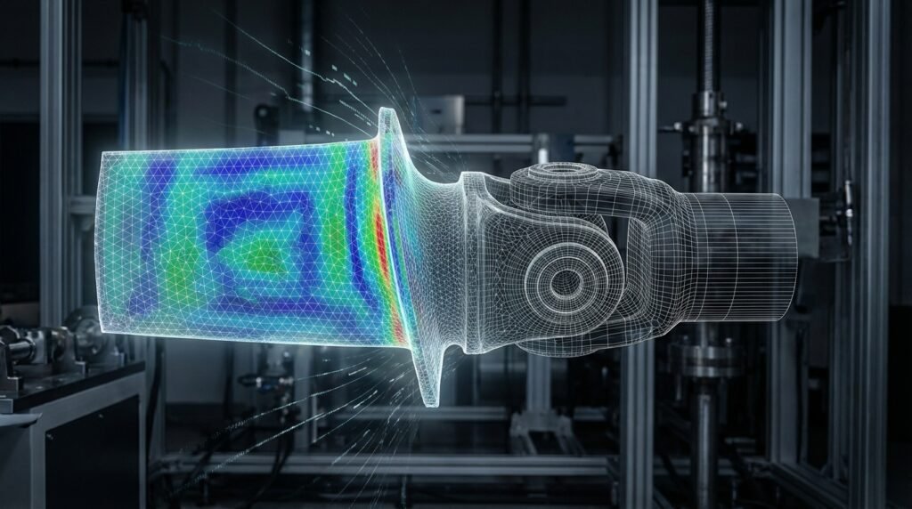
Image: Illustrative LES simulation of turbulent flow past a circular cylinder.

What is Turbulence Modeling?

Turbulence modeling refers to the set of computational approaches used to predict the effects of turbulent fluid flow. Turbulent flows are characterized by chaotic, unsteady, three-dimensional vortices spanning a wide range of length and time scales. Directly simulating every one of these scales (a technique called Direct Numerical Simulation or DNS) is computationally prohibitive for most engineering problems.

Instead, turbulence models introduce approximations or simplifications that allow us to capture the macroscopic effects of turbulence without resolving every microscopic detail. These models are crucial for closing the system of Navier-Stokes equations, which govern fluid motion, when dealing with turbulent regimes.

Why is Turbulence Modeling Essential for Engineers?

Accurate prediction of turbulent flow is vital across numerous engineering disciplines:

• Aerospace Engineering: Designing efficient airfoils, wings, and jet engines requires understanding drag, lift, and heat transfer in turbulent boundary layers.
• Oil & Gas: Predicting pressure drop in pipelines, optimizing pump and valve designs, and simulating mixing processes in reactors.
• Automotive: Reducing aerodynamic drag for fuel efficiency, optimizing engine combustion, and improving cabin ventilation.
• Biomechanics: Analyzing blood flow in arteries (e.g., predicting plaque buildup), designing prosthetic heart valves, and understanding respiratory airflow.
• Civil & Environmental Engineering: Simulating pollutant dispersion, river flows, and wind loading on structures.
• Process Engineering: Optimizing industrial mixing, heat exchangers, and chemical reactors.

Without robust turbulence models, CFD results would often be inaccurate, leading to suboptimal designs, increased prototyping costs, and potential failures in real-world applications. They are integral to CAD-CAE workflows, allowing design iterations to be virtually tested and refined.

Key Categories of Turbulence Models

Turbulence models can be broadly categorized based on their approach to resolving turbulent scales:

1. Reynolds-Averaged Navier-Stokes (RANS) Models

RANS models are the most widely used in industrial CFD due to their computational efficiency. They average the Navier-Stokes equations over time, treating turbulent fluctuations statistically. This introduces new terms, known as the Reynolds stresses, which must be modeled to close the equations. Most RANS models rely on the Boussinesq hypothesis, relating the Reynolds stresses to the mean strain rate via an eddy viscosity.

Common RANS Models:

• k-epsilon (k-ε) Model:
  • Standard k-ε: Robust and widely used, but struggles with adverse pressure gradients and flows with strong swirl/separation. Good for many industrial flows, like internal pipe flow or simple external aerodynamics.
  • Realizable k-ε: Improves upon the standard model by satisfying certain mathematical constraints for Reynolds stresses, performing better for flows with separation and complex secondary flows.
  • RNG k-ε: Derived from renormalization group theory, it’s suitable for rapidly strained flows, swirling flows, and those with strong streamline curvature.
• k-omega (k-ω) Model:
  • Standard k-ω: Excellent for boundary layers and flows with adverse pressure gradients. Sensitive to free-stream conditions, which can be a drawback.
  • SST k-ω (Shear Stress Transport): A hybrid model combining the strengths of k-ε in the far-field and k-ω near the wall. Widely regarded as the best general-purpose RANS model for external aerodynamics, turbomachinery, and flows with separation. It’s often the first choice for complex applications in ANSYS Fluent/CFX and OpenFOAM.
• Reynolds Stress Model (RSM):
  • Directly solves transport equations for all six independent Reynolds stress components. More computationally expensive than eddy-viscosity models but can capture anisotropic turbulence effects more accurately. Useful for highly complex 3D flows, strong swirl, or rotating systems where eddy-viscosity models fall short.

2. Large Eddy Simulation (LES) Models

LES models resolve the large, energy-containing turbulent eddies directly, while only modeling the small, isotropic eddies (subgrid-scale, SGS). This approach is more computationally expensive than RANS but provides more detailed, time-dependent flow information, making it suitable for unsteady flows where transient behavior is critical (e.g., aeroacoustics, combustion, specific FFS Level 3 assessments involving fatigue). Popular SGS models include Smagorinsky and WALE.

3. Direct Numerical Simulation (DNS)

DNS directly solves the Navier-Stokes equations without any turbulence models, resolving all turbulent scales down to the Kolmogorov micro-scales. This is extremely computationally intensive, requiring highly refined meshes and small time steps. Currently, DNS is primarily used for fundamental research and for developing/validating other turbulence models, rather than for routine engineering design.

4. Hybrid RANS-LES Models (e.g., DES, IDDES)

These models combine the computational efficiency of RANS in near-wall regions with the higher accuracy of LES in detached or separated flow regions. They offer a promising compromise for problems requiring high fidelity in specific areas without the full computational cost of LES. Detached Eddy Simulation (DES) and Improved Delayed Detached Eddy Simulation (IDDES) are common examples.

Choosing the Right Turbulence Model: A Practical Guide

Selecting the appropriate turbulence model is crucial for obtaining accurate and reliable CFD results. Here’s a checklist for making your decision:

Factors to Consider:

1. Flow Type:
   • Simple shear flows, boundary layers (no separation): k-ε, k-ω
   • Flows with separation, adverse pressure gradients, swirl: SST k-ω, Realizable k-ε, RSM, LES (if unsteadiness is key)
   • Compressible flows, heat transfer: SST k-ω, Realizable k-ε
   • Rotating machinery, strong anisotropy: RSM
2. Required Accuracy & Detail:
   • Engineering trends, initial design: RANS (k-ε, k-ω SST)
   • Detailed unsteady phenomena, aeroacoustics: LES, Hybrid RANS-LES
   • Fundamental research, model validation: DNS
3. Computational Resources & Time:
   • Limited resources, quick turnaround: RANS (fastest)
   • Moderate resources, good fidelity: Hybrid RANS-LES
   • High-performance computing, long run times: LES, DNS (most expensive)
4. Near-Wall Treatment:
   • Wall Functions: Used with RANS models (e.g., standard k-ε, standard k-ω) when the mesh is too coarse to resolve the viscous sublayer. Less accurate but computationally cheaper.
   • Low-Reynolds Number Models (Wall-Resolved): Requires a very fine mesh near the wall (y+ ~ 1) to directly resolve the viscous sublayer. More accurate but much more computationally expensive. SST k-ω is often used in a wall-resolved manner.
5. Software Capabilities: Familiarize yourself with the strengths and weaknesses of models within your chosen CFD software (e.g., ANSYS Fluent, ANSYS CFX, OpenFOAM).

Turbulence Model Comparison Table (Illustrative)

Model Type	Key Characteristics	Pros	Cons	Typical Use Cases
k-epsilon (RANS)	Two-equation, eddy viscosity	Robust, computationally cheap, good for fully turbulent flows	Poor for adverse pressure gradients, swirl, separation; sensitive to wall treatment	Pipe flow, internal ducts, simple external aerodynamics
k-omega SST (RANS)	Two-equation, eddy viscosity, hybrid k-ε/k-ω	Excellent for boundary layers, adverse pressure gradients, separation; good overall performer	More complex, slightly higher computational cost than k-ε	Aerospace (airfoils), turbomachinery, external vehicle aerodynamics, FFS assessments
Reynolds Stress Model (RSM)	Seven equations for Reynolds stresses	Captures anisotropic turbulence, strong swirl, complex 3D effects	Very computationally expensive, convergence can be challenging	Swirling flows, rotating systems, complex industrial mixing
LES	Directly resolves large eddies, models subgrid scale	High fidelity, captures unsteady phenomena	Very computationally expensive, requires fine mesh and small time steps	Aeroacoustics, combustion, high-fidelity transient analysis
Hybrid RANS-LES (e.g., DES)	RANS near wall, LES away from wall	Balance of accuracy and computational cost	Transition region can be problematic, still more expensive than RANS	Flows with significant separation zones (e.g., bluff bodies, some turbomachinery)

Practical Workflow for Turbulence Modeling in CFD

Implementing turbulence modeling effectively within your CFD workflow requires careful attention to detail, from meshing to post-processing. Here’s a step-by-step approach:

1. Geometry Preparation & Meshing

• CAD Cleanup: Ensure your CAD model is clean and watertight. Tools like CATIA, SolidWorks, or SpaceClaim are commonly used.
• Domain Definition: Create an appropriate computational domain, especially for external flows, to minimize boundary effects.
• Mesh Generation:
  • Boundary Layers: Crucial for turbulent flows. Use inflation layers (prism or hex layers) near walls to accurately capture velocity and temperature gradients.
  • Y+ (Y-plus): This dimensionless wall distance is paramount. For wall-resolved models (e.g., SST k-ω with no wall functions), aim for y+ ≈ 1. For wall-function approaches (e.g., standard k-ε), target y+ between 30 and 300. Mismatched y+ can lead to significant errors.
  • Mesh Refinement: Refine mesh in regions of high gradients (e.g., wakes, shear layers, separation points) and where flow features are critical.

2. Solver Setup

• Fluid Properties: Define density, viscosity, and other relevant properties.
• Boundary Conditions (BCs): Accurately specify inlets, outlets, walls (e.g., no-slip), symmetry planes, etc. For turbulent inlets, specify turbulence intensity and length scale or eddy viscosity ratio.
• Turbulence Model Selection: Based on the guidelines above, choose your primary and perhaps a secondary model for comparison.
• Solver Settings: Select appropriate numerical schemes (e.g., second-order upwind for momentum and turbulence), pressure-velocity coupling (SIMPLE, COUPLED), and under-relaxation factors.

3. Initialization & Solution

• Initialization: Initialize the flow field (e.g., from an inlet, or a previous steady-state solution for transient runs).
• Running the Solver: Monitor convergence carefully.

Verification & Sanity Checks for Turbulence Models

Trusting your CFD results blindly is a common pitfall. Always perform verification and sanity checks:

• Convergence: Ensure residuals drop several orders of magnitude (typically to 1e-4 or 1e-5 for turbulence equations). Monitor key output parameters (e.g., lift, drag, pressure drop) to confirm they reach a steady state or a statistically steady state for transient simulations.
• Grid Sensitivity Analysis: Run your simulation on at least three different mesh resolutions (coarse, medium, fine). If the results change significantly between medium and fine, your mesh is likely too coarse. This is paramount for turbulence models, especially near walls.
• Y+ Monitoring: Always inspect the wall y+ distribution. Ensure it aligns with your chosen near-wall treatment strategy.
• Turbulence Variable Distribution: Visualize contours of turbulent kinetic energy (k) and dissipation rate (ε) or specific dissipation rate (ω). Look for physically plausible distributions and avoid non-physical spikes or zeros in regions where turbulence should exist.
• Velocity Profiles: Compare simulated velocity profiles in boundary layers or wakes with analytical solutions (if available) or experimental data.
• Pressure Distribution: Check for realistic pressure contours, especially in regions of flow separation or reattachment.
• Energy Balance: For conjugate heat transfer problems, verify energy balance at interfaces.
• Boundary Condition Impact: Test sensitivity to inlet turbulence parameters.
• Physical Plausibility: Does the flow field make sense given your engineering intuition?

For complex cases, consider cross-validation with a different turbulence model or even a different CFD solver (e.g., comparing ANSYS Fluent results with OpenFOAM). If you need expert guidance on setting up complex CFD simulations, remember that EngineeringDownloads.com offers specialized online consultancy and tutoring services to help you validate your models and streamline your analysis.

Common Mistakes and Troubleshooting

• Incorrect Y+ Values: The most frequent error. Leads to wrong shear stress and heat transfer predictions. Always check y+ carefully.
• Poor Mesh Quality: Skewness, aspect ratio, and orthogonality issues can lead to convergence difficulties or inaccurate results.
• Inappropriate Turbulence Model Selection: Using k-ε for flows with strong separation or reverse pressure gradients where SST k-ω would be more appropriate.
• Unrealistic Inlet Turbulence: Guessing high turbulence intensity or a very small length scale can lead to rapid turbulent decay or unrealistic predictions downstream.
• Convergence Issues: Often linked to poor mesh quality, high aspect ratio cells, or aggressive solver settings. Start with robust first-order schemes and gradually switch to higher order.
• Misinterpreting Averaged Results: RANS models provide time-averaged results. Don’t expect to see instantaneous vortex shedding, which requires LES or DNS.
• Lack of Validation Data: Always try to compare your simulation results with experimental data, analytical solutions, or other trusted benchmarks if available.

Leveraging Tools and Automation

Modern CFD software packages like ANSYS Fluent, ANSYS CFX, and OpenFOAM offer a wide array of turbulence models and robust solvers. For pre-processing and post-processing, tools like ANSYS SpaceClaim, ANSYS Meshing, Tecplot, and ParaView are invaluable.

For automating repetitive tasks, running parametric studies, or integrating CFD into larger CAD-CAE workflows, scripting with Python or MATLAB is highly effective. You can automate mesh generation (e.g., with Python scripts for OpenFOAM’s snappyHexMesh or Fluent’s TUI), modify boundary conditions, run simulations, and extract specific results. For instance, a Python script could run a series of simulations with varying turbulence model parameters to assess sensitivity.

Further Reading

For more in-depth theoretical understanding and specific model details, refer to authoritative resources like NASA’s Turbulence Modeling Resource:

NASA Langley Research Center – Turbulence Modeling Resource

Frequently Asked Questions (FAQ)

What is the difference between RANS, LES, and DNS?

RANS (Reynolds-Averaged Navier-Stokes) models average turbulent fluctuations, providing time-averaged results at low computational cost. LES (Large Eddy Simulation) directly resolves large eddies and models only the small ones, offering more detail at a higher cost. DNS (Direct Numerical Simulation) resolves all turbulent scales directly, providing the highest fidelity but is computationally prohibitive for most engineering applications.

When should I use the SST k-omega model?

The SST k-omega (SST k-ω) model is often recommended as a good general-purpose RANS model. It performs particularly well for flows with adverse pressure gradients, flow separation, and in regions where accurate boundary layer predictions are crucial, such as external aerodynamics, turbomachinery, and many industrial applications.

What is y+ and why is it important in turbulence modeling?

Y+ (y-plus) is a dimensionless wall distance that determines the location of the first computational cell away from a wall relative to the viscous sublayer. It is critical because different turbulence models and near-wall treatments require specific y+ ranges for accurate results. For wall-resolved models, y+ should be near 1, while for wall-function approaches, it typically needs to be between 30 and 300.

Can I simulate transient phenomena with a RANS model?

While RANS models are time-averaged, they can be run in a ‘unsteady RANS’ (URANS) mode to capture large-scale, low-frequency unsteadiness (e.g., vortex shedding for certain geometries). However, URANS does not resolve the full spectrum of turbulent fluctuations; for high-fidelity transient turbulence, LES or hybrid RANS-LES models are more appropriate.

Are turbulence models applicable to all fluids?

Most common turbulence models are developed for Newtonian fluids. While the fundamental principles can be adapted, applying them directly to non-Newtonian fluids often requires specific modifications to the viscosity term or specialized models that account for shear-thinning, viscoelasticity, or other complex rheological behaviors.