Columns are the backbone of many structures. they support roofs, floors, and beams, keeping buildings and bridges standing strong. In construction, steel and concrete are two primary materials for columns. Each has its advantages: steel is extremely strong and ductile (bends rather than breaks), while concrete is excellent in compression and can be reinforced with steel rebars for tension. Often, they’re combined as reinforced concrete (RC) or composite steel-concrete columns to get the best of both worlds. But how do engineers ensure these columns won’t crack, buckle, or fail under heavy loads? This is where finite element analysis (FEA) comes into play. Using advanced simulation tools like Abaqus, Ansys, or OpenSees, we can virtually test steel and concrete columns under various conditions – from everyday gravity loads to earthquakes and blasts – before ever building them in real life.

In this blog, we’ll explore how to model steel and concrete columns in FEA, with a focus on Abaqus (one of the most powerful FEA tools available). We’ll discuss the unique behavior of each material, how to represent reinforcement, and techniques for simulating critical phenomena like buckling, cracking, and composite action. We’ll also touch on other tools (like Ansys and OpenSees) and why FEA is so crucial for column design in both academic research and industry practice. By the end, you’ll have a clear picture of the key steps and considerations for simulating steel and concrete columns – and how our EngineeringDownloads team leverages these techniques in our projects and training package.

(As an aside, if you’re eager for hands-on guidance, our Steel and Concrete Columns Package in Abaqus offers 25+ step-by-step tutorials covering everything from basic RC column modeling to advanced scenarios like composite columns under blasts and cyclic loads[1]. But for now, let’s dive into the core concepts!)

Understanding Steel vs. Concrete Columns

Steel columns are usually made of rolled steel sections (like I-beams, hollow tubes, or angles) and are prized for their high strength-to-weight ratio. Steel behaves in a ductile manner: it will typically yield (deform plastically) before it fails, giving visible warning (bends) rather than sudden collapse. However, a big concern for slender steel members is buckling – under compression, a tall thin steel column can suddenly bow sideways and lose strength even if the material hasn’t yielded. The tendency to buckle depends on the column’s length, cross-section, and end support conditions. For example, a column fixed at both ends is more resistant to buckling than one that’s pinned or free at one end. In design, we characterize this by an effective length factor K (related to end conditions) and use Euler’s critical load formula to estimate buckling load. Steel columns can also face local buckling (flanges or walls of the section buckling locally) if they’re thin-walled. Despite these challenges, steel’s predictability (well-defined yield point and stress-strain curve) makes it relatively straightforward to model in FEA.

Concrete columns, on the other hand, are made of a brittle matrix (concrete) usually combined with steel reinforcement bars (rebars) to carry tension. Plain concrete is very strong in compression but weak in tension – it can crack easily once tensile stress exceeds its low tensile strength. That’s why nearly all concrete columns are reinforced concrete (RC) columns: vertical steel rebars take tension and control cracking, while horizontal ties (stirrups) hold the rebars in place and provide confinement. An RC column’s behavior is complex and nonlinear: under load, concrete will crack in tension, and eventually crush in compression if overstressed; steel rebars will yield in tension; and the interaction between steel and concrete (bond and slip) can affect stiffness. If not properly confined, even the steel rebars in a concrete column can buckle within the concrete when the concrete cracks or spalls off under extreme load. Despite concrete’s complexity, it’s ubiquitous in construction due to its cost-effectiveness and compressive strength.

Composite columns combine steel and concrete in a single member in a more integrated way than normal RC. For example, a concrete-filled steel tube (CFST) uses a steel hollow section filled with concrete – the steel jacket provides confinement to the concrete and carries tension, while the concrete core increases compressive capacity and prevents the thin steel tube from buckling inward. Another example is a steel-reinforced concrete column, where a wide-flange steel shape is embedded in a concrete column (often used in high-rises). These composite designs have excellent strength and ductility, but modeling them means you have to capture two materials interacting together (with possible slip at the interface if not perfectly bonded).

Understanding these differences is important because it dictates how we set up our simulations. Steel’s main concerns are yielding and buckling; concrete’s are cracking, crushing, and the steel-concrete bond. Now, let’s see why FEA is the go-to method to analyze these behaviors.

Why Use Finite Element Analysis for Columns?

Traditionally, engineers use formulas and building codes to design columns. For instance, Euler’s formula gives the critical buckling load for an ideal column, and concrete design codes give empirical formulas for load capacity (taking into account reinforcement ratios, concrete strength, etc.). While these analytical methods are great for quick estimates and design checks, they have limitations. Real columns may have irregular geometry, material inhomogeneities, or complex loading that defy simple formulas. Moreover, once a column goes into the nonlinear range (beyond yield or when concrete cracks), analytical solutions become very hard. This is where finite element analysis shines.

FEA allows us to break a complex column into many small elements and simulate how each piece behaves under stress. This means we can capture local effects (like stress concentrations, cracking patterns, or local buckling waves) and global behavior (overall deflection, load capacity) in one model. For example, FEA can simulate the progressive formation of cracks in a concrete column and how those cracks reduce stiffness, something that’s nearly impossible to do with hand calculations. It can also predict the post-buckling deformation of a steel column or the load redistribution when one material yields before the other.

Another big reason to use FEA is to avoid or complement physical experiments. Physical testing of columns (like crushing a full-scale concrete column or performing a cyclic load test) is expensive, time-consuming, and sometimes impractical. Numerical simulation is a cost-effective alternative to explore “what-if” scenarios. Researchers often employ FEA to test new designs or materials (e.g., what if we add 10% more steel? what if the concrete is ultra-high-strength? what if an explosion impacts the column?). As one study notes, while experiments provide crucial insights, they require enormous time and cost, so numerical methods (like FEA) have become increasingly popular for understanding concrete behavior. In industry, FEA helps refine designs before construction, leading to safer and more efficient structures.

FEA is also invaluable for investigating failures and edge cases. Think of scenarios like: How will a particular RC bridge column behave in a magnitude 7 earthquake? Will a certain steel column design survive a fire or an explosion? What is the factor of safety if some corrosion has reduced the steel area? By simulating these situations, engineers can design mitigation (like adding wraps to a column for seismic retrofit) or choose better materials.

To sum up, FEA provides a virtual testing lab for steel and concrete columns. It complements classical analysis by handling the messy, nonlinear, and coupled behaviors that real structures exhibit. Modern software packages come with extensive material models and features tailored for these tasks – and among them, Abaqus is a top choice for many engineers due to its powerful concrete and steel modeling capabilities. In the next sections, we’ll focus on how to set up column models in Abaqus (though the principles carry over to other tools like Ansys and OpenSees as well).

Simulation Tools and Approaches for Column Modeling

Before diving into specifics, it’s worth noting how different FEA tools approach steel and concrete column simulation:

• Abaqus: A versatile FEA software known for its robust material models. Abaqus has a built-in Concrete Damage Plasticity (CDP) model for concrete that captures cracking and crushing behavior with damage accumulation. It also offers metal plasticity models with options for isotropic or kinematic hardening, and criteria for ductile damage (to simulate fracture in steel). Abaqus supports various element types (beams, shells, solids) and powerful contact definitions – useful for composite interactions or rebar embedding. Because of its breadth, we’ll use Abaqus as the reference for most methods described here.
• ANSYS: Another widely used FEA tool. ANSYS has traditionally offered a element type called SOLID65 specifically for concrete, which, paired with its “CONCRETE” material model, can simulate concrete cracking and crushing. In ANSYS Workbench, you can also use nonlinear material models (Drucker-Prager, etc.) for concrete and rebar definition in a similar spirit to Abaqus. ANSYS can handle reinforcement either by smeared approaches or discrete rebar objects. It may not have a one-click CDP model like Abaqus, but it provides the building blocks to achieve similar results. (Notably, ANSYS now also has advanced concrete models like the Microplane model with element CPT215 to address some limitations of SOLID65.)
• OpenSees: An open-source simulation tool specifically geared towards structural and earthquake engineering. OpenSees is different – it uses a fiber section approach for columns and beams in many cases. Instead of 3D solid elements, you often model a column as a line element with a cross-sectional fiber model (each fiber having concrete or steel material behavior). This allows efficient nonlinear analysis of frame structures under cyclic loads. OpenSees has many specialized material models for reinforcement, confined concrete, etc., calibrated for seismic response. For example, in OpenSees one would simulate an RC column by using a nonlinear beam-column element with a fiber section that includes concrete (cover and core) and steel fibers; this captures the axial-flexural behavior and P-M interaction well. However, OpenSees won’t directly give you a 3D crack pattern – it’s more for global response and hysteresis. It’s commonly used in academia for performance-based earthquake simulations.

Each tool has its strengths: Abaqus for detailed continuum analysis, ANSYS for robust general FEA with some concrete specialization, OpenSees for structural-level simulations of structures under dynamic loads. Regardless of tool, the fundamental steps to model a column are similar – define geometry, assign material behavior, apply interactions or constraints (especially for composite sections), mesh it, and apply loads/boundary conditions. Let’s go step by step, focusing on the Abaqus approach for clarity.

Modeling Steel Columns in Abaqus (and Other FEA Tools)

Simulating a steel column in Abaqus is often one of the simpler tasks in FEA, but it still requires careful attention to certain details. Here’s a roadmap for modeling a steel column:

1. Geometry and Element Type: Decide how to represent the column. If the column is prismatic (constant cross-section) and you’re mainly interested in overall behavior (like buckling load or deflection), you might use beam elements (line elements with assigned section properties). Beam elements in Abaqus capture axial, bending, and even torsional behavior efficiently. However, if local buckling or detailed stress distribution is of interest (say the column walls buckling or connection details), you’d use shell elements (for thin-walled steel sections) or solid elements (for thick sections or to capture 3D effects). For example, an H-shaped wide-flange column could be modeled with shell elements representing its flanges and web; a solid rod column could be one solid part.
2. Material Model for Steel: Steel’s behavior can be defined as elastic-plastic. In Abaqus CAE, you’ll specify a plasticity model with the yield stress (fy) and either a plastic hardening curve or a simple bilinear approximation. By default, this is an isotropic hardening model (the yield surface expands uniformly after yielding). If you plan to do cyclic loading, you might opt for combined isotropic/kinematic hardening to capture the Bauschinger effect (where the yield stress in compression vs tension can differ after reversal due to internal stress re-distribution). Abaqus also allows adding a ductile damage initiation criterion – this predicts onset of fracture when a certain plastic strain (often a function of stress triaxiality and strain rate) is reached. For most design simulations, you might not need to go as far as simulating fracture, but it’s good to know Abaqus can do it if required (for example, simulating a steel column snapping due to an explosion or impact).
3. Boundary Conditions: How the column ends are supported has a huge impact on results. You can fix the base, free or pin the top, etc., just as in a real structure. For buckling analysis, you’d likely simulate idealized conditions: pinned ends can be modeled by allowing rotation (no moment fixity) at the ends, while fixed ends have all rotations constrained. Abaqus can do this by applying appropriate encastre (fixed) or releasing rotations with connector elements or coupling constraints. It’s important to match the boundary conditions to whatever scenario you are analyzing (for example, a column in a moment frame has a stiff beam at top – not a free end).

 

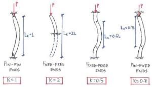
Figure: Effective length factor (K) for various column end conditions, which influences buckling. A pin-pin column has K≈1 (half-sine wave buckling shape, effective length = actual length L). A fixed-free (cantilever) column is more prone to buckling, K≈2 (effective length is about 2L). A fixed-fixed column is more restrained, K≈0.5, and a pinned-fixed column K≈0.7. These factors modify the critical buckling load: more restraint (lower K) means higher buckling capacity. In FEA, you simulate these by adjusting end supports accordingly, as illustrated above.

4. Buckling Analysis (if needed): If you want to find the buckling load/capacity of the steel column, a common approach is to perform an eigenvalue buckling analysis first. In Abaqus, you can run a Linear Buckling step, which will output mode shapes (the predicted buckling shapes) and associated eigenvalues – these eigenvalues can be multiplied by the applied load to estimate the theoretical buckling load. The lowest eigenvalue corresponds to the weakest buckling mode (e.g., the first-mode buckling shape). Note that eigenvalue buckling assumes perfect geometry and purely elastic behavior, so it often overestimates buckling load in practice. Engineers usually introduce small imperfections into the model (by deforming the mesh slightly in the shape of the buckling mode) and then run a nonlinear analysis to see the real buckling with material yielding. Imperfections account for real-world crookedness or initial imperfections and help trigger buckling in the simulation at a lower load, more in line with tests. In any case, FEA gives you a visual of the buckling mode shape, which is helpful in understanding how the column might deform (e.g., sway in the middle, double-curvature, etc.). And as noted, boundary conditions set the mode shape; for example, the FEA might show a half-sine deflected shape for a pin-pin column versus a quarter-sine for a fixed-free.
5. Nonlinear Static Analysis: To simulate the actual load-bearing including yielding, you set up a static step (or dynamic if needed) where you gradually increase axial load (and maybe lateral load if checking combined loading) on the column. In Abaqus Standard, you might use Static Riks or Static General with stabilization if expecting an instability. The Riks method (arc-length) is great for tracing post-buckling behavior because it can handle the load dropping after peak (snap-through or collapse), which normal force-control might not capture once the column loses capacity. You’d apply the load at the top (e.g., a concentrated force or distributed pressure on a cap plate). As load increases, monitor displacement and stress. The column will typically go elastic, then yield (if steel yields), and at some point exhibit large lateral deflection if buckling kicks in. FEA will capture the interaction of material yielding and geometric nonlinearity, which is important because for many steel columns, the critical load might be reached with some material yielding (inelastic buckling).
6. Results Interpretation: From the FEA results, you would check the axial load vs axial shortening curve, lateral deflection, stress distribution in the cross-section, etc. If the simulation includes post-yield, you might see the formation of a plastic hinge at mid-height (for slender columns that buckle in the middle) or at the ends. For stocky columns, you might see the material fully yielding across the section (squash load) without buckling. Modern FEA can also reveal if local buckling occurs, say if using shell elements you might see the flange locally wrinkle. You should correlate the FEA-predicted ultimate load with design code predictions to ensure consistency and safety margins.

A quick comparison to other tools: If doing this in ANSYS, the workflow is similar – perform an eigenvalue buckling (ANSYS Linear Buckling analysis) then a nonlinear analysis with imperfections. ANSYS’s SOLID65 concrete element isn’t relevant for a pure steel column; instead, you’d use shell elements (e.g., SHELL181) or beam elements and define bilinear isotropic hardening for steel. In OpenSees, one might not explicitly do eigen buckling; instead, you would assign an initial geometric imperfection and run a nonlinear push (OpenSees can simulate geometric nonlinearity if you use nonlinear beam-column elements with multiple integration points). OpenSees would require you to provide a yield curve for steel (it has Steel01, Steel02 material models, etc. for steel fibers with kinematic hardening options for cyclic). The concept of buckling in OpenSees for a single column would come from the geometric instability of the element if modeled as a column with several elements and initial bow imperfection. So, while the tools differ, the physics is the same – you need to introduce what makes the column buckle and you need a material model for yielding.

Connections: Often a steel column isn’t isolated – it connects to beams or a footing. If your model includes part of a frame, Abaqus can simulate bolt or weld connections (using connector elements or contact). For simplicity in a column-alone model, you might assume either fixed or pinned ends. But if you’re interested in connection behavior (say a bolted column-base plate), you can include that in the FEA with contact for bolts, etc. This goes beyond just the column itself but is crucial in many practical simulations (our team has, for instance, simulated steel beam-column connections with bolts in Abaqusto examine how connection slip and bolt preload affect column behavior).

Lastly, failure of a steel column can be assessed by criteria such as exceeding a certain plastic rotation or by using the ductile damage model to delete elements upon fracture. Abaqus allows element deletion once a damage criterion reaches a value of 1, which can simulate a tearing failure. This is more commonly used in extreme blast or impact simulations.

In summary, to model a steel column: define the geometry, assign steel’s elastic-plastic (and possibly damage) behavior, set realistic boundary conditions, consider performing a buckling analysis or adding imperfections, then ramp up loads to see how it behaves. With Abaqus, you’ll be able to capture both yielding and instability. And importantly, FEA results can strongly correlate with classical theory – for example, Dlubal’s study showed FEA and Euler’s buckling load differed by barely 1% in many cases when ideal conditions were modeled[13] (of course, real life has imperfections which we include via the methods discussed).

Modeling Reinforced Concrete Columns in Abaqus

Concrete is a more challenging material to simulate because of its nonlinear and brittle nature. Abaqus provides a powerful tool for this: the Concrete Damage Plasticity (CDP) model. Let’s break down how to model an RC column (reinforced concrete column) step by step:

1. Geometry and Meshing: Typically, an RC column is modeled with 3D solid elements for the concrete (e.g., C3D8 hexahedral elements) and either embedded elements or truss elements for the steel rebars. You’ll draw the column’s cross-section (usually rectangular or circular) and extrude it to the column height. If you plan to include discrete rebars, you’ll sketch lines for each rebar and assign them a separate part (which can be 2-node line elements of type Truss or Wire region). An alternative approach is to use embedded rebar layers within a solid or shell section, which we’ll discuss shortly. Mesh the concrete with a reasonably fine mesh around the rebar regions to capture stress concentrations at steel-concrete interface. Keep an eye on aspect ratios and try to have a symmetric mesh if the column is symmetric.
2. Concrete Material Model (CDP): Abaqus’s Concrete Damage Plasticity model is an all-in-one constitutive law that covers cracking in tension and crushing in compression with damage evolution. In simpler terms, it assumes concrete has a plasticity component (non-recoverable strain) and a damage component (reducing stiffness after cracking/crushing). The CDP model requires a bunch of parameters: elastic modulus E and Poisson’s ratio ν (for initial linear behavior), the compressive yield (or failure) curve, the tensile cracking behavior (often given by a tensile strength and fracture energy for softening), and other shape parameters like the dilation angle, stress ratio (flow potential eccentricity), etc. It might sound daunting, but many of these have default or recommended values (Abaqus documentation or literature provides typical CDP parameters for different concrete strengths). Essentially, CDP combines two failure mechanisms – tensile cracking and compressive crushing – into one model. Before running the analysis, double-check that the stress-strain data you input (especially the post-peak softening for tension and compression) is realistic for your concrete (too brittle can cause convergence issues, too ductile would be non-conservative).

Under the hood, CDP is an isotropic hardening plasticity model derived from Drucker-Prager theory, augmented with scalar damage variables for stiffness degradation. For example, when the concrete cracks in tension, CDP will reduce the effective stiffness in that direction gradually (tension stiffening effect can be defined so that after cracking, the concrete still carries some tension via rebar bond until completely fractured). In compression, after the peak, the model reduces stiffness to simulate crushing. The beauty of CDP is that it can capture nonlinear behaviors like stiffness degradation under cyclic loading, different responses under multiaxial stress states, etc., without needing user-written subroutines. (If needed, Abaqus also has other simpler models – e.g., Brittle Cracking or Drucker-Prager without damage – but CDP is generally the go-to for RC simulation.)

3. Steel Reinforcement Modeling: Now we need to include the steel bars in the concrete. There are two common ways to do this in Abaqus, depending on the type of elements used for concrete:

• Embedded Region method (discrete rebar): In this approach, you explicitly model the rebars as separate wire/truss elements and “embed” them in the concrete solid mesh. Abaqus will internally constrain the degrees of freedom of the rebar nodes to the surrounding concrete element interpolation (essentially tying them, so they move with the concrete). This is great for 3D detailed models[16]. You can allow some slip by adjusting constraints or using surface-based interactions instead, but in its basic form, the Embedded Region ties them perfectly (assuming a good bond). The advantage is you get a realistic representation of rebar placement, and you can even get output like rebar stress directly. This method is essential if you have complex rebar arrangements (stirrups, multiple layers, etc.) and want to study things like bond-slip (which would require a more advanced contact definition or connector elements to simulate slip). In research, it’s noted that capturing the bond-slip effect between steel and concrete is crucial for realistic results, and the embedded approach (with proper contact modeling) can do that better than smeared rebar layers. In our experience, if bond-slip is critical, one might use surface-to-surface contact with cohesive behavior between a beam/shell representation of rebar and concrete, but that’s a pretty advanced setup. Most often, an embedded constraint with a slightly adjusted modulus can approximate bond behavior.
• Rebar Layer in Elements (smeared reinforcement): If your column is prismatic and especially if using shell or membrane elements (like modeling a wall or thin section), Abaqus lets you define rebar as layers within the element properties. This is a “smeared” approach – you don’t draw each bar; instead, you tell Abaqus that, say, in this concrete section there is a layer of steel at a certain depth with X mm^2 area per meter, spaced at certain intervals. It’s very useful for 2D simulations or when you want to avoid modeling each bar in 3D (which can add a lot of mesh complexity). The rebar layer approach assumes perfect bond (the strain in the rebar layer is pulled from the concrete strain), and it’s typically limited to relatively low reinforcement ratios (Abaqus recommends it for cases where the reinforcement volume is small and distributed, e.g., 1–4% by volume). In a column, that’s usually fine because columns often have reinforcement in that range. One limitation is that this approach can’t capture localized effects like bar slip or bar buckling – it’s an averaged effect. But it greatly simplifies modeling since you don’t need separate rebar mesh. For a straight column under pure compression, a smeared rebar might be adequate. For something like a beam-column joint or an area with anchorage, discrete rebars are better.

Both methods can even be combined in advanced models (e.g., smeared longitudinal bars plus discrete hoops), but that’s rarely necessary. In summary, use embedded discrete rebar for higher fidelity; use rebar layers for simplicity when detailed bar behavior isn’t critical.

4. Boundary Conditions and Loads: Similar to the steel column, you set the support conditions for the concrete column. Often the base is fixed (encastre), and the top might have a load applied via either a distributed pressure on a loading platen or a prescribed displacement if doing a displacement-controlled test simulation. For concentric compression tests, I like to apply displacement at the top to capture the post-peak descending branch (since force-controlled would drop off once it cracks/crushes). For eccentric loading or bending, you’d apply lateral loads or moments. Just ensure to avoid unrealistic fixity if, say, the column in reality would crack at the ends – sometimes analysts add rigid end blocks (with a stiff elastic material) to simulate the presence of a top and bottom stub that don’t crush, which helps focus damage in the column length.
5. Analysis Steps: You might simply do a static general step, but concrete models often need stabilization or smooth loading because once cracking starts, there can be convergence difficulty (due to stiffness degradation). Using Static Riks could capture the softening post-peak (if, for example, the column crushes and can’t carry as much load, Riks can follow that drop). Another technique is to apply load under displacement control gradually. If doing cyclic loads (for seismic), you would do multiple steps of push and pull, or use an Amplitude curve to modulate a displacement boundary condition back-and-forth. Keep an eye on energy outputs (dissipated energy in damage, etc.) to see that the solution is stable.
6. Outputs and Interpretation: Key things to look at are the crack patterns (Abaqus can output “STATUS OF DAMAGE” or discrete cracks if using the old smeared crack approach – but with CDP, it’s more continuous damage variables dt and dc for tension and compression damage). You can visualize where tension damage is 1.0 (fully cracked) to see how cracks distributed (often diagonal cracks for shear or vertical splitting cracks if they occur). Check the load-displacement curve of the column – typically an RC column will exhibit a peak load then a softening (due to concrete crushing or rebar yielding and buckling). If confinement (stirrups) is modeled, you may see a more ductile response (slower softening). The stress in rebars is another output – you want to see if steel yielded (e.g., rebar stress hitting yield plateau). Concrete compressive stresses can go up to f’c then soften. Often, a simulation will show concrete in the core still carrying stress while cover concrete might have cracked and lost capacity, which is realistic.

From our own simulations and those of others, a well-calibrated concrete model in Abaqus can match physical test results impressively well. For example, one can match the load-axial deformation curve of a tested RC column within a few percentage points by adjusting the tensile fracture energy and post-peak behavior. This builds confidence that the model captures the essential physics.

Reinforcement considerations: If using the embedded approach, realize that by default Abaqus ties the rebar and concrete perfectly. Real RC columns may have slip, especially if anchors aren’t perfect. To simulate bond-slip rigorously, one approach is to use connector elements (with elasticity/plasticity) between the rebar nodes and equivalent positions in concrete, representing the bond shear stiffness and possible slip. There is also research where people use interface elements or cohesive elements for rebar. But unless you have specific data on bond-slip, an easier approximation is to slightly reduce rebar stiffness after yield to mimic loss of bond (or just be aware the model might be a bit stiffer pre-cracking than reality due to perfect bond assumption).

Alternate software notes: In ANSYS, as mentioned, SOLID65 is a common element for concrete. You can assign multilinear isotropic material for concrete in compression and define a cracking criterion (ANSYS requires input of cracking/shear transfer coefficients, etc.). Rebars in ANSYS can be modeled as embedded “rebar elements” within SOLID65 (similar to Abaqus rebar layers concept) or as discrete LINK180 elements. ANSYS’s Concrete model and SOLID65 can track cracking in specific orientations (up to three cracks at a node). It’s a bit of an older formulation, but many have used it successfully. Interestingly, ANSYS even warns that the SOLID65+Concrete material combo is mesh-sensitive (results can vary with mesh density) – a known issue with concrete softening behavior unless regularized. Abaqus’s CDP tends to have some mesh sensitivity too (as any damage model does), so using a fracture energy approach (as CDP does) helps ensure energy is dissipated per crack area, making it less mesh-dependent.

In OpenSees, you wouldn’t model a single concrete column with 3D continuum elements (it’s possible via some tcl scripting and using their FEAPI, but not typical). Instead, you’d likely model it as a column element with a fiber section. The concrete in fibers can use models like Concrete01 (Kent-Scott-Park model with crushing), Concrete02 (with tensile strength and linear tension softening), etc., and steel fibers use Steel02 (Giuffré-Menegotto-Pinto model with kinematic hardening, very popular for seismic). Fiber sections inherently consider axial-moment interaction and you can assign confinement effects by using different stress-strain for core concrete vs cover (accounting for stirrup confinement in the core). OpenSees fiber models won’t directly show a “crack”, but when you see the curvature localizing or a drop in the force, that’s analogous to a major crack forming or the rebar yielding. Also, for dynamic analysis, OpenSees can do time-history analysis on a column (for instance, apply an earthquake motion at the base to see how the column behaves).

Wrapping up the RC column modeling: The combination of Abaqus CDP model for concrete + embedded rebar is a powerful way to simulate RC columns. It captures the key behaviors: cracking (with tension stiffening), yielding of steel, interaction between steel and concrete, and even cyclic degradation if you reverse load. It’s always wise to validate the model with a known experiment – for example, simulate a well-documented column test from the literature to ensure your material parameters are calibrated. Once validated, you can use the model to explore new designs or conditions, such as how adding FRP wraps will increase strength (you can add shell elements around the concrete with a composite material for CFRP and tie them, to simulate a wrapped column), or how a higher-strength concrete (with different CDP inputs) will change the failure mode.

Composite Columns and Special Cases

Composite steel-concrete columns come in several flavors. Let’s discuss two common types and how to model them, as well as some special scenarios like retrofitting:

1. Concrete-Filled Steel Tubes (CFST): This is a circular or rectangular hollow steel tube filled with concrete. These are popular in high-rise buildings and bridges because the steel tube provides confinement and formwork for the concrete, and the concrete prevents local buckling of the tube from the inside. To model a CFST in Abaqus, you’d create two parts: a shell (or solid) for the steel tube and a solid for the concrete core. The critical aspect is the interface between steel and concrete. You have choices: assume perfect bond (tie the contact surfaces together) or allow slip and separation (define a contact interaction). In reality, bond might be good until slip occurs at higher loads or if the steel yields. A common approach is to tie them for simplicity, which assumes no slip and no gap – the composite will act fully together (this usually overestimates stiffness a bit but is conservative for strength). A more advanced approach is to use surface-to-surface contact with a frictional formulation: normal behavior “hard” contact (no penetration) and tangential behavior with a friction coefficient to allow some sliding. If you expect debonding, you could even use a cohesive zone model for the interface.

Abaqus can handle either method. If using surface contact, you mesh the steel and concrete such that their surfaces match or are reasonably compatible, then define an interaction. This can capture phenomena like the steel tube slightly slipping or the concrete shrinking away if it cracks (losing contact pressure). Research has shown that accurately modeling the steel-concrete interaction is crucial for composite columns– it influences load transfer and confinement. For instance, if the bond is too low, the steel might carry more tension and the concrete more compression until they start to slip.

Material-wise, you’ll assign the steel tube a metal plasticity model (and maybe damage if expecting fracture in the tube under extreme load). The concrete core uses CDP as before. In a CFST under axial compression, the failure might occur by the steel tube yielding/buckling outward and the concrete crushing inside. Confinement can enhance concrete strength (which you could include in the CDP parameters by increasing the effective f’c due to the steel hoop stress). Some advanced models even use a different concrete stress-strain for confined concrete (the CDP model can be calibrated for confinement by tweaking dilation angle and flow potential eccentricity, or simply input a higher compressive strength/strain capacity).

When you run the analysis (e.g., compressing the composite column), look at both materials: you might see the steel tube’s hoop stress become significant (indicating it’s confining the concrete). If the steel tube is thin, you might see local buckling bulges outward between contact points (which FEA can capture if using shell elements and if mesh is fine enough to allow a half-wave buckle shape). Indeed, in one FEA study of CFST, the FEA showed local outward bulging of the steel wall, matching test observations. You can also track the Mises stress in steel and the concrete’s principal stresses – a contour plot of Mises stress might show high stress rings near the ends (due to load introduction) and mid-height (due to column effective length).

 

 

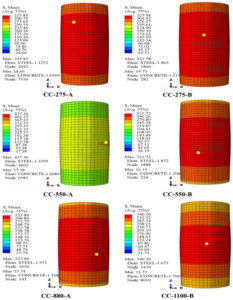
Figure: Von Mises stress distribution in various concrete-filled steel tube (CFST) column models under axial compression (Abaqus FEA results, adapted from open-access study). The steel tube (outer shell) and concrete core (inside) work together to carry the load, as seen by the distribution of stress across both materials. Red regions indicate high stress (approaching yield in the steel); they occur near the loaded ends and mid-height, while the concrete core shows a more uniform stress sharing. Such FEA contour plots help engineers visualize how composite action distributes forces in a column.

To verify composite action, one can compare the FEA-predicted capacity to a calculated value (there are code formulas for composite column strength, or one can sum the steel yield load plus concrete ultimate load considering confinement). FEA often gives insight into failure mode: whether it’s dominated by steel yielding or concrete crushing or instability.

2. Encased or Built-Up Composite Columns: Consider a steel I-section embedded in a concrete column, or a concrete column jacketed with a steel plate. Modeling these follows the same principles: include both materials, tie or contact their interface, and assign appropriate material laws. An encased steel shape in concrete might be fully bonded (often they have shear connectors in reality to prevent slip). So you could tie the steel shape nodes to the concrete, or use embedded region constraint treating the steel shape as “rebar” (but it’s 2D extensive, so better to tie surfaces). If the steel is a dense shape (taking significant area), realize that the concrete around it is somewhat confined but also reduced in area. So adjust the concrete material if needed for confinement.

One thing to watch: if using shells for steel and solids for concrete, tie constraints between shell edges and solid faces can be tricky – you might need to create a surface on the shell (shell thickness can be considered or use a Shell-to-solid coupling feature in Abaqus). Abaqus has a feature specifically to connect shells to solid faces that ensures compatible deformation.

3. Retrofitting with FRP or Steel Jackets: A common industrial application is strengthening an existing concrete column by wrapping it with fiber-reinforced polymer (FRP) sheets or adding a steel jacket. To simulate an FRP-wrapped column, you can add a thin shell around the column diameter, assign it an orthotropic elastic material (or elastic-plastic if it’s some ductile material) to represent the FRP. For FRP, usually it’s linear elastic until brittle failure; you could set a failure strain at which you remove the elements to simulate rupture of the wrap. The FRP shell is tied to the concrete surface (assuming good bond using epoxy). This will confine the concrete as load increases, effectively raising its strength. FEA will show the FRP primarily carrying hoop tension (you can check stress in the wrap). Our team has looked at scenarios like spiral FRP strips wrapping a column – in FEA you might model those as individual narrow strips of shell with gaps in between to see if spacing matters. Indeed, spiral CFRP wraps and other retrofits are topics we cover in our training, demonstrating how adding such elements in the model increases column ductility.

If a steel jacket is added (say a steel tube around an old concrete column), that becomes like a CFST (with an initial gap maybe if not tight). You can simulate the gap by not tying initially and allowing contact closure.

4. Seismic Considerations (hysteresis and confinement): Under cyclic loading, composite columns can be very complex. For instance, in a cyclic lateral loading test on a CFST, the steel will yield back and forth and the concrete core might degrade gradually. Abaqus can capture Bauschinger in steel (with kinematic hardening) and stiffness degradation in concrete (with damage accumulation in CDP). However, sometimes specialized models (e.g., in OpenSees, there’s a specific “ConcreteFM” for fiber models with confinement and slip, etc.) are used to match cyclic loops precisely. If one is focusing on seismic performance, fiber models in OpenSees are efficient for slender columns in frames, while Abaqus continuum models can better capture things like bar buckling or out-of-plane deformation if the column deteriorates.

One special case: reinforcement bar buckling inside an RC column under compression – Abaqus can capture this if you explicitly model the bar and maybe introduce an initial imperfection in the bar and have ties (stirrups) providing lateral support at intervals. You’d then see in analysis, between tie points, the bar might buckle out of the concrete once concrete cover is gone. This is advanced but has been studied; it explains why ties spacing is limited by codes (to prevent rebar buckling out between them).

5. Thermal and Fire effects: Though not requested explicitly, sometimes one might simulate a column under fire (thermal expansion causing internal stress). Abaqus can do coupled temperature-displacement analysis. Steel loses strength with temperature, concrete spalls at high temp – those can be included via temperature-dependent material properties and an element death or discrete spall model. Tools like Ansys have dedicated procedures for fire analysis of columns. It’s a niche but important in design for robustness.
6. Dynamic impact or blast in composite columns: If, say, a column is subjected to an impact load or blast, strain rate effects become important. Concrete and steel can resist higher stresses at high strain rates (a phenomenon called dynamic increase factor, DIF). Abaqus’s CDP doesn’t automatically include strain rate effects, but you can implement them by scaling strength based on strain rate in an Abaqus/Explicit analysis, or by using other material models. For example, the Johnson-Holmquist (JH-2) model is often used for concrete under high-rate loads (penetration, explosions). Abaqus includes the JH-2 model (keyword Concrete Johnson-Holmquist) specifically for such cases. JH-2 is a sophisticated model that accounts for damage accumulation in a different way and is tuned for high pressures and strain rates (originally developed for ceramics and concrete under impact). If our composite column was subject to a blast, we might use Abaqus/Explicit, assign JH-2 to concrete, and perhaps Johnson-Cook plasticity to steel (which accounts for strain rate hardening in metals). We’d apply a blast load either as a pressure-time curve on the surfaces or simulate the blast wave with a CEL (Coupled Eulerian-Lagrangian) approach where the air and explosive are modeled to impinge on the column, or with SPH particles to simulate the blast pressures. These techniques let the shock wave interact realistically with the structure, at the cost of more simulation complexity. They’re quite advanced, but they are exactly the kind of high-end simulations our team has tackled in our course/projects, for example modeling an explosion on an RC column wrapped with CFRP and analyzing damage.

To illustrate, in one tutorial we demonstrate applying a TNT blast load to a RC column model: using SPH for the explosive and CDP for concrete, we captured the scabbing of concrete and the fracture of rebars. Without FEA, it would be guesswork to predict such violent responses. With FEA, you can literally see a simulation of the column fragmenting or surviving, and tweak designs (maybe a thicker jacket or more ties) to improve outcome.

7. Summary of Our Training Package Topics: Throughout this blog, we touched on many advanced topics – and if it feels like a lot, don’t worry. Mastering these techniques takes practice. At EngineeringDownloads, we’ve created a comprehensive training package that guides you through all these scenarios step by step. Our Steel and Concrete Columns Simulation package covers everything from basic academics to industry applications. For instance, we include workshops on: standard RC column compression tests, RC composite columns (with steel profiles inside), pure steel columns under cyclic bending, concrete-filled steel tubes under load, columns strengthened with CFRP wraps, seismic analysis with cyclic lateral loading and hysteresis loops, blast analysis using CEL and SPH methods, buckling and post-buckling of slender columns, and material modeling with CDP, JH-2 (for impact), ductile damage in steel, and more. It’s a treasure trove for those who want to become experts in column simulation – essentially condensing years of experience into guided examples. Whether you’re a grad student researching new composite columns or an industry engineer checking a difficult design case, these simulations can be a game-changer in how you approach column design and analysis.

Advanced Analysis: Seismic and Blast Loading on Columns

Thus far, we’ve mostly discussed static or monotonic loading. Two of the most demanding load cases for columns are earthquakes (seismic) and blasts (explosive impacts). These deserve special attention in simulation:

Seismic (Cyclic) Loading: During earthquakes, columns experience rapidly reversing loads – one moment a column might be in tension (being pulled as the building sways), the next moment in compression, along with bending back and forth. This causes low-cycle fatigue and cumulative damage. For steel columns, repeated cycles can lead to Bauschinger effects (reduced yield on reversal) and eventual fracture if cracks develop. Abaqus can simulate cyclic plasticity by using the Combined Hardening model (mixing kinematic hardening for the Bauschinger effect with isotropic for overall growth of yield surface). You would apply a cyclic displacement history to the top of the column (say, push one direction to a drift ratio, pull the other, and so on). The results would be hysteresis loops (plots of lateral force vs displacement) showing pinching or strength degradation if damage is included. For RC columns, cyclic loads will open and close cracks – this is where the damage parameter in CDP evolves. Each crack reopening is a bit easier (stiffness has dropped), so the second cycle might have less stiffness than the first – matching what we see in experiments (hysteresis loops that degrade). Also, confinement by hoops in RC columns is crucial under cyclic loads to prevent bar buckling and to maintain some ductility; in FEA, if you explicitly model the hoops, you might see they yield in tension during outward deformation and provide pressure on concrete when it tries to expand in compression.

OpenSees is heavily used for simulating such cyclic response because it has specific models for cyclic degradation (you can include stiffness and strength degradation parameters in some materials). But Abaqus with CDP can also capture a lot of it naturally through the damage formulation. One should be careful with convergence in cyclic analyses – as unloading and reloading can cause sudden stiffness changes when cracks close or reopen. Sometimes using a small viscosity in CDP (a damping term in the constitutive equations) helps.

After simulating a cyclic test, you might extract things like the energy dissipation per cycle, the drop in strength after a number of cycles, etc. These are important for performance-based design (e.g., did the column survive 3% drift with acceptable residual strength?).

Blast and Impact: We touched on this in composite column context, but generally, for blast Abaqus/Explicit is the tool. The steps are: define the blast load (either via a pressure load using empirical blast curves or an actual modeling of the explosion), use appropriate high-rate material models (or at least increase material strengths based on expected strain rates), and very small time increments (explicit time integration with maybe mass scaling if needed for speed). The output is usually the maximum deflection of the column, whether it breaks (elements erode if using damage criteria), and the impulse it transmits to the rest of the structure.

For example, suppose we want to see if a concrete column in a parking garage can withstand a certain bomb blast. We’d model the column, perhaps using CDP for concrete but we should increase f’c for high strain rate (since concrete strength can double under blast strain rates – we could do this via defining a Rate Dependent tab in CDP or manually scaling strength). Or we switch to JH-2 which inherently accounts for strain rate by formula. We’d model the blast by placing an Eulerian domain around the column with high-pressure initial conditions to simulate the explosive, etc., or just apply an equivalent pressure pulse of, say, X MPa for Y milliseconds based on standards. The Abaqus output might show the column spalling – you’d see damage variable = 1 near the explosion side, indicating concrete is fully damaged there. Rebars might snap if the strain exceeds their capacity (you could allow element deletion for rebar if damage > 1). If the column fails in the simulation (e.g., gets cut in half), that’s a serious result – it means in reality, collapse could occur. Then you might try a retrofit in simulation: wrap the column with a steel jacket or FRP and simulate again to see if it holds together (the jacket would catch pieces and provide confinement). We actually walk through such scenarios in our advanced tutorials, demonstrating how different materials behave under blasts and how combined systems (steel + concrete + composites) can provide resilience.

It’s fascinating that FEA predictions have been confirmed by experiments in these extreme cases. For instance, when comparing simulated and experimental deformed shapes of blast-loaded composite columns, one study found very good agreement. This gives engineers confidence to use simulation for scenarios where testing is not feasible (you can’t exactly set off large blasts repeatedly to test every design!).

Other Special Cases: We could also mention creep and shrinkage (long-term effects on concrete columns) – Abaqus can do creep via user-defined visco models or implicit creep laws, which would be relevant for, say, a concrete column under sustained load to see deformation over years. Or soil-structure interaction if a column is in the ground (pile behavior) – Abaqus can incorporate soil via springs or continuum elements with Drucker-Prager models.

But these might be beyond the scope of this already expansive discussion. The key point is, whether it’s monotonic loading to failure, cyclic earthquake loading, or blast impact, modern FEA tools can simulate the column’s response with a high degree of realism. The insights gained help engineers design safer structures (e.g., deciding stirrup spacing for seismic columns, or adding jackets for blast protection).

Conclusion

Steel and concrete columns are fundamental elements in structures, and getting their design right is paramount for safety. Through this exploration, we’ve seen that finite element simulation is an invaluable tool in an engineer’s arsenal for understanding column behavior under various scenarios. Steel columns require careful attention to buckling and yielding; concrete columns demand modeling of cracking, crushing, and reinforcement interaction. With FEA, we can capture phenomena like a steel column’s sudden buckling under critical load, or the progressive cracking and strength loss in a concrete column as load increases. We can even anticipate complex behaviors in composite columns, where steel and concrete act together to carry loads.

Crucially, simulations allow us to push the limits: we can subject virtual columns to earthquakes, blasts, fire, or any extreme event and see how they fare. This predictive power means we can iterate designs – maybe increase the rebar here, add an FRP wrap there – all in the computer, to find an optimal solution before implementing it in the real world. It also helps forensic investigations (why a column might have failed in an accident) and informs updates to design codes.

Our journey touched on a broad range of topics: material models (from basic elastic-plastic to sophisticated damage models), modeling techniques (embedded rebars, contact interfaces), and load cases (static, cyclic, dynamic). If it feels overwhelming, remember that with practice and the right guidance, each piece falls into place. We at EngineeringDownloads are passionate about sharing this know-how. That’s why we developed our Steel & Concrete Columns Simulation course – to help engineers and researchers gain practical experience in these simulations, backed by theory. We’ve distilled years of expertise into example problems and tutorials so you can learn by doing, from academic fundamentals to real industrial applications. Check out our Steel and Concrete Columns Package in Abaqus on website.

 

Whether you’re aiming to ace a graduate thesis on novel concrete composites or ensuring a high-rise building’s columns meet safety margins, the combination of solid theory and advanced FEA will give you a competitive edge. And if you ever feel stuck or have a unique column problem to solve, remember that we also offer consulting services – our team is ready to assist in setting up models, interpreting results, or even developing custom simulation methodologies for your project.

In the end, the goal is simple: build safer, more efficient, and innovative structures. By leveraging tools like Abaqus (and others) for virtual testing, we can push the boundaries of what’s possible with steel and concrete, all while keeping risk low in the real world. We hope this comprehensive overview has demystified some of the process and inspired you to incorporate simulation in your workflow.

Thank you for reading, and happy simulating!

Written by Pille Nurm.