Resolving Singular Matrix Errors in Engineering Simulations

troubleshooting
Engineering Downlaods
April 9, 2026
21 Minute

As engineers navigating the complexities of numerical simulations – whether it’s Finite Element Analysis (FEA), Computational Fluid Dynamics (CFD), or structural integrity assessments – encountering a ‘Singular Matrix Error’ can be a frustrating roadblock. This isn’t just a cryptic message; it’s your solver’s way of telling you that your model, as it stands, is mathematically ill-posed. Essentially, it implies that the system of equations it’s trying to solve either has no unique solution or an infinite number of solutions.

This comprehensive guide is designed to demystify singular matrix errors, providing you with actionable insights, troubleshooting steps, and best practices to ensure your engineering models are robust and solvable. We’ll cut through the academic jargon and deliver practical, engineer-to-engineer advice.

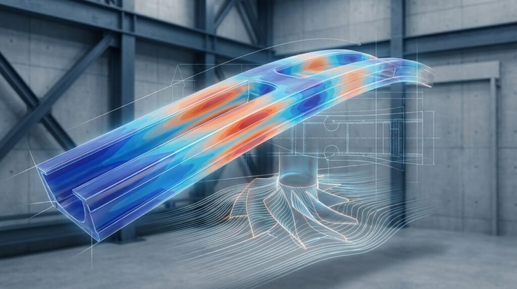
Image by Krishprasad and H. A. R. R., via Wikimedia Commons, depicting a basic truss structure often used in structural analysis demonstrations.

Understanding the Core Problem: What is a Singular Matrix?

Before we dive into solutions, let’s establish a foundational understanding of what a singular matrix signifies in the context of engineering analysis.

Mathematical Intuition

In linear algebra, a square matrix ‘A’ is considered singular if its determinant is zero. Practically, this means that the matrix does not have an inverse. When solving a system of linear equations of the form Ax = b (where ‘A’ is your system matrix, ‘x’ is the vector of unknowns, and ‘b’ is the known load/source vector), a singular ‘A’ implies that a unique solution for ‘x’ cannot be found. This could mean either no solution exists or infinitely many solutions exist, leading to solver failure.

Engineering Context: The Stiffness Matrix (FEA) / System Matrix (CFD)

In FEA, the system matrix is often referred to as the global stiffness matrix [K], and the system solved is typically [K]{u} = {F}, where {u} are the nodal displacements and {F} are the applied forces. In CFD, a similar system arises from discretized Navier-Stokes equations, with the system matrix representing the coupled fluid properties and the unknown vector typically containing velocities and pressures.

A singular stiffness matrix [K] indicates that your structure or component has at least one ‘rigid body motion’ mode or an unconstrained degree of freedom (DOF). Imagine a free-floating object in space; you can apply a force, but there’s no unique displacement because it can translate or rotate indefinitely without resistance. The solver cannot compute a unique displacement field, leading to the error.

Analogy: The Unconstrained Structure

Think of a table with only two legs on a perfectly smooth floor. If you push it, it will slide and spin indefinitely. It’s ‘unconstrained’ and has too many degrees of freedom for a unique static position. A singular matrix error is the mathematical equivalent of this situation in your numerical model.

Common Causes of Singular Matrix Errors in Engineering Simulations

Understanding the root causes is the first step toward effective troubleshooting. Here are the most frequent culprits:

Inadequate Boundary Conditions (BCs)

This is by far the most common reason for a singular matrix error, especially in structural and solid mechanics problems.

Under-Constraining the Model

Lack of Restraint: The model is not adequately fixed in space. For a 3D structure, you need to constrain at least six degrees of freedom (three translations, three rotations) to prevent rigid body motion. Even if you only care about deflections in one direction, the other directions must be appropriately constrained.
Incorrect DOF Fixation: Sometimes, engineers apply constraints, but they don’t cover all necessary DOFs. For instance, fixing only translation but allowing rotation at a point that should be fully pinned.
‘Floppy’ Structures: Sometimes components are connected but too ‘flexible’ or have incorrect connections, allowing local rigid body motion within a larger assembly.

Incorrectly Applied Constraints

Over-Constraining (Redundant BCs): While less common for singularity, applying redundant BCs can lead to other solver issues or stress concentrations. However, if two BCs contradict each other, it can cause problems.
Weak Springs: In some solvers like MSC Nastran, ‘weak springs’ are used to stabilize models. If they are too weak or applied incorrectly, they may not prevent rigid body motion.

Material Properties & Element Behavior

Errors here can make your model mathematically unsolvable.

Zero or Negative Material Properties

Zero Stiffness: If Young’s Modulus (E) is zero, the material has no stiffness, and any part made of it will behave like a mechanism, leading to singularity.
Negative Properties: Negative Young’s Modulus or Poisson’s Ratio (if outside physically allowable range) can result in a non-positive definite stiffness matrix, leading to mathematical instability.

Incompatible Elements

Element Type Mismatch: Using elements not suitable for the physics (e.g., using beam elements where shell elements are needed, or vice-versa) can lead to local instabilities if connections aren’t correctly handled.

Geometric Issues

Flaws in the CAD model or meshing can manifest as singular matrices.

Disconnected Meshes (Free Floating Parts)

Unconnected Components: If two parts in an assembly are intended to be connected but are not due to meshing gaps or incorrect contact definitions, one part might be ‘floating’ in space relative to the other.
Zero-Area/Volume Elements: Degenerate elements (e.g., a 3D solid element collapsing into a 2D face or 1D line, or a 2D shell collapsing into a 1D line) have zero stiffness contribution, causing local singularity. This often happens with poor CAD cleanup or aggressive meshing parameters.

Rigid Body Motion

Mechanisms: If your assembly inherently forms a mechanism (like an unconstrained linkage system), the model will exhibit rigid body motion until appropriate constraints or kinematic couplings are applied. This is common in multi-body dynamics simulations using tools like ADAMS.

Solver and Numerical Instabilities

While often a symptom of model setup, sometimes solver settings play a role.

Poorly Conditioned Matrices

Vastly Different Stiffnesses: A model with extremely stiff components connected to extremely flexible components can lead to a system matrix that is numerically ill-conditioned. While not strictly singular, it can be close enough to cause solver difficulties.

Contact Issues

Initial Penetrations/Gaps: Incorrect initial contact conditions can sometimes lead to a singular matrix, especially if a part is ‘supported’ only by contact that hasn’t been established correctly in the initial step.

Practical Workflow for Diagnosing and Resolving Singular Matrix Errors

Here’s a step-by-step approach to track down and fix these elusive errors, applicable across tools like Abaqus, ANSYS Mechanical, MSC Patran/Nastran, and even Python/MATLAB scripts for custom solvers.

Step 1: Understand the Error Message

Your solver’s output is your best friend. Don’t just dismiss it. Look for keywords like ‘rigid body motion detected’, ‘pivot point’, ‘zero pivot’, ‘unconstrained DOFs’, or references to specific nodes or elements.

Tool-Specific Messages

Abaqus: Often reports ‘zero pivot’ at a specific degree of freedom of a node, or ‘numerical singularity’. Look for messages about the global stiffness matrix being unstable.
ANSYS Mechanical: Messages like ‘singular matrix detected’ or ‘large negative pivot’. The output often points to the first detected singularity, which might be a symptom rather than the primary cause.
MSC Nastran: Look for ‘FATAL ERROR U.M. 4292’ or messages related to ‘singular stiffness matrix’ and a list of ‘dependent DOFs’.
MATLAB/Python: If you’re building your own solver, the error will likely come from the matrix inversion or decomposition function (e.g., numpy.linalg.inv, scipy.linalg.solve).

Step 2: Boundary Condition Check (The First Suspect)

This is almost always the first place to look. Systematically go through your constraints.

Visual Inspection: Use your pre-processor (e.g., ANSYS Workbench, Abaqus/CAE, Patran) to visually inspect every applied boundary condition. Are they where you think they are?
DOF Coverage: For a 3D static analysis, ensure your model is constrained against translation in X, Y, Z and rotation about X, Y, Z. You don’t necessarily need to fix all 6 DOFs at a single point, but the combination of all BCs must restrain all rigid body motions.
Symmetry Conditions: If using symmetry, ensure the plane of symmetry correctly constrains perpendicular translations and in-plane rotations.
Smallest Possible Constraints: Use minimal constraints that prevent rigid body motion. Over-constraining can introduce unrealistic stresses. A common technique is to fix one point fully (all 6 DOFs), another point for 2 DOFs (e.g., Y and Z translation) and a third point for 1 DOF (e.g., Z translation), forming a ‘tripod’ support.
Incremental Application: If unsure, start with a fully fixed model (all external nodes fixed) and gradually remove constraints until the minimum set is found.

Step 3: Geometry and Mesh Inspection

After BCs, geometry and mesh quality are critical.

Check for Disconnected Components: Use assembly tools in your pre-processor to check for unintended gaps between parts. Use ‘merge nodes’ or ‘equivalence’ functions to connect coincident nodes if necessary.
Inspect Element Quality: Look for distorted, degenerate, or collapsed elements. Most pre-processors have tools to highlight elements with poor aspect ratios, Jacobian values, or skewness. Re-mesh problematic areas with finer control.
Free Edges/Faces: For solid models, ensure there are no unintended free edges or faces internally, which can indicate poor meshing or a gap.
Small Gaps/Overlaps: Tiny gaps or penetrations in CAD can lead to meshing issues or contact errors that cause singularity. Clean your CAD geometry rigorously.

Step 4: Material Property Verification

A quick sanity check for material properties is crucial.

Positive Values: Ensure Young’s Modulus, Shear Modulus, and Poisson’s Ratio (within -1 to 0.5 for isotropic materials) are positive and physically realistic.
Consistent Units: Verify that all material properties, geometry, and loads are in a consistent unit system.

Step 5: Contact Definition Review

If your model involves contact, scrutinize its setup.

Initial Status: Are parts initially touching, or is there a gap? For small gaps, some solvers can ‘bond’ surfaces, but significant gaps can lead to one part being unconstrained until contact is established.
Contact Type: Is the contact type appropriate (e.g., ‘bonded’, ‘no separation’, ‘frictionless’, ‘frictional’)? Incorrect contact can effectively create unconstrained mechanisms.
Contact Stabilisation: Some solvers offer stabilization methods (e.g., contact damping or small ‘penalty’ stiffnesses) which can help with initial contact but shouldn’t mask fundamental BC issues.

Step 6: Solver Settings & Advanced Diagnostics

In rare cases, solver settings might contribute, or advanced diagnostics can pinpoint the issue.

Automatic Stabilization: Some solvers offer automatic ‘stabilization’ options for static analysis (e.g., Abaqus’s *STABILIZE parameter). These add a minimal stiffness to prevent rigid body motion, allowing the solution to proceed. While useful for complex contact, they should not replace proper BCs.
Eigenvalue Analysis: Perform a normal modes (eigenvalue) analysis. If you have rigid body modes (eigenvalues very close to zero), it explicitly confirms unconstrained DOFs. This is an excellent diagnostic tool.
Subtle, Helpful CTA: For models with particularly complex contact or highly non-linear behavior, resolving singular matrix errors can be time-consuming. EngineeringDownloads.com offers tutoring and online consultancy services, providing expert guidance to efficiently troubleshoot and optimize your simulations.

Common Cause Category	Typical Manifestation	Troubleshooting & Resolution
Boundary Conditions (BCs)	Model ‘flies off’, zero pivot, no constraint in one or more DOFs.	Visually inspect BCs. Ensure minimum 6 DOFs (3 trans, 3 rot) are constrained for 3D. Use minimal set of BCs. Perform normal modes analysis to find rigid body modes.
Geometry & Mesh	Disconnected parts, degenerate elements, poor element quality.	Check for free-floating components. Merge nodes. Inspect mesh quality; re-mesh problematic areas. Clean up CAD geometry to remove small features or gaps.
Material Properties	Zero or negative stiffness values.	Verify all material properties are positive and physically realistic. Ensure consistent unit system.
Contact Definitions	Initial penetrations/gaps, incorrect contact type creating a mechanism.	Review initial contact status. Adjust contact settings (e.g., initial adjustment for small gaps). Use contact stabilization if appropriate, but sparingly.
Numerical Instability	Highly disparate stiffnesses, very small loads on large models.	Check for large differences in component stiffness. Scale loads if too small. Consider explicit dynamics for highly non-linear problems if implicit struggles.

Prevention is Better Than Cure: Best Practices for Robust Models

Implementing these practices from the outset can significantly reduce the likelihood of encountering singular matrix errors.

Initial Model Setup Checklist

Sketch BCs: Before even opening the software, sketch your structure and intended BCs. How will it be constrained in the real world?
Simplification First: Start with a simplified model. Apply rough loads and BCs to ensure it runs without singularity before adding complexity.
Review Default Settings: Understand the default contact and meshing settings of your software (Abaqus, ANSYS, etc.).

Progressive Loading and Analysis

For complex non-linear problems (material non-linearity, large deformation, contact), apply loads incrementally:

Start with linear analysis to verify model stability.
Gradually introduce non-linearity (e.g., small loads, then full loads; frictionless contact, then frictional).
This helps isolate the source of error if one arises.

Using Appropriate Element Types

Select elements that are suitable for your geometry and expected deformation modes. For instance:

Shell elements: For thin-walled structures.
Solid elements: For bulky components.
Beam elements: For slender members.
Be mindful of element order (linear vs. quadratic) and integration (reduced vs. full).

Python and MATLAB for Pre-Processing Checks

For advanced users, scripting languages can be powerful for preventative checks:

Mesh Quality Scripts: Python scripts (e.g., using libraries like meshio or solver APIs) can automate checking element quality metrics across large models.
Stiffness Matrix Conditioning: In MATLAB or Python (with NumPy/SciPy), you can assemble a simplified stiffness matrix and check its condition number (numpy.linalg.cond). A very high condition number indicates a nearly singular matrix. This is excellent for academic or custom FEA solvers.
Automatic BC Generation: For repetitive tasks, Python scripts can ensure consistent application of boundary conditions. EngineeringDownloads.com offers a library of downloadable Python scripts and MATLAB functions to streamline your pre-processing and verification workflows.

Verification & Sanity Checks for Post-Resolution Confidence

Once you’ve resolved the singular matrix error, don’t just move on. Verify the results to ensure your fix didn’t introduce new problems or unrealistic behavior.

Displacement and Stress Fields

Visual Review: Plot displacement contours. Do they make physical sense? Are displacements concentrated where expected? Are there any ‘hot spots’ of excessive, unrealistic deformation?
Magnitude Check: Are the magnitudes of displacements reasonable for the applied loads and material stiffness?
Stress Distribution: Check stress contours. Are stresses concentrated at expected locations (e.g., corners, holes)? Are there any unrealistic stress singularities (often caused by point loads or sharp corners not handled correctly)?

Reaction Forces

Equilibrium Check: Sum the reaction forces at your boundary conditions. Do they balance the applied external loads? This is a fundamental check for overall equilibrium.

Energy Balance

Strain Energy: Most solvers report strain energy. Is it positive? A negative strain energy indicates a serious problem, potentially with material definitions or element formulation.
Kinetic Energy: In implicit static analysis, kinetic energy should ideally be zero or negligible. High kinetic energy might indicate dynamic effects if not properly suppressed or an unstable solution.

Sensitivity Analysis

If your model is sensitive to slight changes in boundary conditions or material properties, it might be an indicator of a poorly conditioned model, even if not strictly singular. Run a few small variations to check robustness.

Engineeringdownloads.com Resources

At EngineeringDownloads.com, we understand the challenges engineers face in complex simulations. Beyond this article, we offer a range of resources to help you master your tools and techniques. Explore our library for downloadable templates, project files, and advanced Python/MATLAB scripts tailored for FEA, CFD, and structural integrity applications. For personalized assistance, our expert tutoring and online consultancy services are available to guide you through your most demanding projects.

Frequently Asked Questions (FAQ)

What does a ‘Singular Matrix Error’ mean in FEA?

In FEA, a singular matrix error typically means that the global stiffness matrix of your model is not invertible. This usually indicates that your structure is not adequately constrained and can undergo ‘rigid body motion’ without any resistance, making it impossible for the solver to find a unique displacement solution.

What are the most common causes of a singular matrix error?

The most common causes include inadequate boundary conditions (under-constraining the model), disconnected geometry or mesh parts, zero or incorrect material properties (e.g., zero Young’s Modulus), and poorly defined contact conditions leading to free-floating components.

How do I fix a singular matrix error in Abaqus or ANSYS?

Start by meticulously checking your boundary conditions to ensure all rigid body motions are constrained. Then, inspect your model’s geometry and mesh for disconnected parts or degenerate elements. Verify material properties are positive and realistic. Finally, review contact definitions for any gaps or incorrect setups. Using a normal modes analysis can help pinpoint unconstrained DOFs.

Can Python or MATLAB help diagnose singular matrix errors?

Yes, especially in custom solvers or for pre-processing. Python with NumPy/SciPy can be used to check the condition number of a stiffness matrix, indicating how close it is to singularity. Python scripts can also automate mesh quality checks and ensure consistent application of boundary conditions in pre-processors via their APIs.

Is a singular matrix error the same as a convergence error?

No, they are distinct. A singular matrix error means the solver cannot even *start* to find a unique solution due to an ill-posed mathematical problem (usually rigid body motion). A convergence error, on the other hand, occurs when the solver *can* initiate a solution but fails to converge to a stable answer within the specified tolerances, often due to highly non-linear behavior, large deformations, or numerical instabilities during iteration.

Can over-constraining cause a singular matrix error?

While over-constraining can lead to other issues like artificial stress concentrations or solver difficulties (especially in non-linear problems), it is generally not a direct cause of a singular matrix error. A singular matrix typically indicates *under-constraining* or a lack of resistance to motion, not too much constraint. However, conflicting boundary conditions could indirectly lead to solver issues that might be mistaken for singularity.

What is a ‘zero pivot’ error?

A ‘zero pivot’ error is a specific type of singular matrix error reported by some solvers (like Abaqus). It occurs during the matrix decomposition process (e.g., Gaussian elimination or LU decomposition) when a zero or near-zero value is encountered on the diagonal of the matrix. This indicates that the corresponding degree of freedom is unconstrained or that the system has become numerically unstable at that point.