Life Assessment and Continuum Damage Creep Analysis of Welded Components

By: Saman Hosseini – Expert in creep welding simulation, fatigue, and FFS Level 3 assessments.

Introduction

Imagine a high-pressure steam pipe in a power plant, with countless welded joints, all enduring red-hot temperatures for decades. How do engineers predict whether those welds will survive or fail over time? This is where creep life assessment comes in – especially crucial for welded components operating at high temperature. In this blog, we’ll explore how experts analyze the creep behavior and damage of complex welded structures using advanced techniques like Continuum Damage Mechanics (CDM) and finite element simulation (in software such as Abaqus and Ansys). We’ll also see how these methods fit into Fitness-For-Service (FFS) Level 3 assessments for critical equipment, and why they matter for industries like oil & gas and nuclear power. Let’s dive in!

What is Creep and Why Welded Components Are at Risk

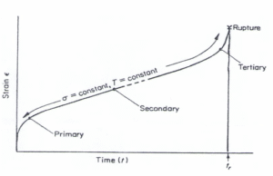
Creep is the time-dependent, slow deformation of materials under stress at elevated temperature. In high-temperature equipment (e.g. furnaces, boilers, reactors), metals can creep – gradually elongating or bending under load long before they actually “break.” Creep typically occurs in three stages: primary (slowing rate), secondary (steady rate), and tertiary (accelerating deformation leading to failure). The tertiary stage is characterized by the formation of micro-voids and cracks, causing a rapid increase in strain until rupture.

 

When it comes to welded components, creep damage tends to be more severe and complex. A weld is not a uniform material – it consists of the weld metal, the base metal, and the heat-affected zone (HAZ) in between, each with different microstructures and creep strengths. Often, the HAZ (especially the fine-grained region adjacent to the weld) is the weak link. In ferritic creep-resistant steels (like the chromium-molybdenum steels used in power plants), a phenomenon called “Type IV” cracking occurs: the HAZ material deteriorates and fails before the base metal, typically with minimal overall deformation across the weld. Essentially, the weld’s HAZ creeps faster and forms cavities or cracks sooner than the rest of the component. Despite improved alloys, many power plants have seen weld failures due to Type IV cracking in the HAZ.

For example, Grade P91 steel (a 9%Cr-1%Mo-V alloy widely used since the 1980s for high-temperature pipes and headers) has exhibited premature creep failures at welds. Field experience showed that P91 weldments sometimes cracked in significantly less than 100,000 hours of service, raising safety and reliability concerns. Evidence suggests that standard design guidelines were overly optimistic (non-conservative) for P91 welds. In other words, the welds became the “weakest link” – creep damage in the welded joints accumulated faster than expected, even though the base metal itself was holding up fine. This mismatch in behavior underscores why we need specialized analysis for welded areas.

What makes welded components tricky in creep: the material properties are heterogeneous, and residual stresses from welding can influence creep (initially accelerating it in some areas until they relax). Creep damage often localizes – for instance, a crack might initiate in a narrow zone of the HAZ while the surrounding material is relatively undamaged. Traditional life estimation methods (like Larson-Miller parameter correlations or simple time-to-rupture charts) do not capture this localization well. Therefore, engineers turn to more advanced methods, like continuum damage mechanics models and finite element analysis, to predict where and when a creep failure might occur in a welded component.

It’s also important to note that if a creep crack has already formed in a component, the assessment approach shifts to fracture mechanics. In creep conditions, cracks can grow steadily over time (creep crack growth). Engineers use parameters like the C* integral to characterize crack growth rate under creep. Procedures such as British Energy’s R5, API 579-1/ASME FFS-1, BS 7910, and others provide guidance for evaluating creep cracks in components. These methods assume a crack is present and predict how long it will take to propagate to a critical size. However, in this blog, our focus is on continuum damage analysis – predicting the initiation of creep damage and overall life of the welded structure before a crack visibly forms. This is a key part of FFS Level 3 assessments to prevent failures in the first place.

Continuum Damage Mechanics (CDM) and Creep Life Prediction

How can we predict creep failure before it happens? Enter Continuum Damage Mechanics. CDM is a framework that introduces a damage variable (often denoted ω) into material constitutive models to represent deterioration. L. M. Kachanov is credited with introducing the CDM concept back in 1958, with the premise that by modeling the kinetics of damage accumulation, one can predict the duration of the tertiary creep stage and thus estimate creep life. In Kachanov’s model, the damage variable ω starts at 0 (no damage) and increases towards 1 (fracture) as creep voids and micro-cracks form in the material. This seminal idea influenced many researchers – Rabotnov, Hayhurst, Lemaitre, and others expanded the approach in subsequent decades. Over time, CDM has become an umbrella for many phenomenological models of creep damage. The core concept, however, remains: instead of just using time or strain as a predictor, we explicitly track damage evolution in the material.

In a creep CDM model, the material’s creep strain rate is coupled to the current damage level. Early on (ω near 0), the creep rate might be low (primary or secondary creep). But as damage builds up (voids reducing load-bearing area, etc.), the creep rate accelerates – capturing the tertiary creep behavior. Eventually, when ω = 1 at a point, it indicates local rupture. By integrating these equations, we can predict not just when a component fails, but also where (the location that first reaches the critical damage). The advantage of CDM is that it can realistically represent that accelerating creep and looming failure which simple models (that only account for secondary creep) would miss.

One practical example of a CDM-based approach is the Omega Method used in industry for creep life assessments. The Omega method essentially models the entire creep process as if it were tertiary creep – it employs a damage parameter Ω that characterizes how fast creep damage accumulates. The mathematics of the Omega method come from continuum damage concepts: it uses an exponential creep law where the creep strain rate increases as a function of stress and damage, in a way that can be fit to short-term test data. In simpler terms, you do some accelerated creep tests, extract an Ω value for the material, and then you can predict long-term creep life by assuming damage grows continuously with strain. The Omega method was developed so that this Ω parameter could be determined from relatively short duration tests, and an extensive materials database was built for it (the MPC Project Omega) which is now part of standards like API 579-1/ASME FFS-1. It’s an engineering approach that gives practitioners a formula to calculate remaining life without doing a full-blown finite element simulation each time.

However, Omega is just one flavor of CDM. It’s actually one example of a general family of continuum damage models originating from Kachanov’s work. Many other CDM models exist (Kachanov-Rabotnov, Hayhurst’s model, ductility exhaustion models, etc.). Industry codes historically did not widely adopt these advanced damage models directly in design rules, precisely because they are not trivial to solve without a computer. They often require iterative or time-stepping analysis (nowadays, that means using FEA). That said, with modern computing power, it’s increasingly feasible to apply CDM in day-to-day fitness-for-service evaluations, especially at Level 3 where high fidelity is desired. In fact, the latest FFS standards do encourage advanced analysis for creep: API 579’s creep assessment recommendations include the Omega method and acknowledge that finite element creep simulation can be used for Level 3 assessments. The bottom line: CDM provides the theoretical foundation to simulate creep damage and life, and with the help of finite element tools, we can bring that theory to bear on real welded components.

Challenges in Creep Life Assessment of Welded Joints

Welded components combine the complexity of material heterogeneity with the demands of high-temperature operation. A few key challenges must be addressed when performing creep life assessment on welds:

• Material Gradients: The weld metal, HAZ, and base metal often have different creep properties (creep strength, ductility, rupture time, etc.). For example, the HAZ in ferritic steel welds can have a tempered martensite or bainite microstructure that creeps faster than the base metal’s fully tempered structure. If one simply used base metal creep data for the whole weldment, predictions would be unconservative. We saw this with Grade 91 steel – the weld HAZ creep strength is lower than the base metal, leading to life overestimations by standard methods. Any realistic life assessment must account for these zone-specific behaviors.
• Type IV Cracking in HAZ: As mentioned, Type IV creep cracking is a well-known failure mode in low alloy and creep-strength-enhanced ferritic steels. This cracking occurs in the intercritical or fine-grain HAZ (often abbreviated FGHAZ), usually after long-term exposure. It’s characterized by many small grain-boundary cavities that coalesce into cracks with relatively little overall strain. Type IV failures effectively shorten the creep life of welded components compared to what you’d expect from tests on base metal specimens. Many failures in power plants have been traced to this mechanism, and it remains an area of active research and concern. For an assessor, this means extra conservatism is needed unless detailed analysis is done – you cannot assume a weld will last as long as an unwelded piece of the same material.
• Residual Stresses and Welding History: Welding leaves residual stresses which can influence creep. Initially, tensile residual stresses in a weld could accelerate creep damage (since creep rate is higher under higher effective stress). Over time, creep itself causes stress relaxation. The net effect is complicated – residual stress might cause early damage in specific regions (e.g. near weld fusion line) before it relaxes. Advanced creep analysis can actually simulate this relaxation. In some cases, a weld’s residual stress will have diminished after a few years of high-temperature service (so it might not affect long-term life much), but in other cases, especially if operating stress is low, residual stress might remain a driving force for damage for a long time. It’s something to consider in a comprehensive assessment.

• Localized Creep Strain and Damage: Unlike a uniform tensile specimen, a welded structure can concentrate creep strain in certain areas. For instance, if one part of the weldment creeps faster (say the HAZ at the inner surface of a pipe weld, where temperature might be a bit higher and material a bit weaker), that area will accumulate damage and might form a creep crack, while other areas are still relatively unharmed. This non-uniform damage means inspection and monitoring should focus on likely hot-spots (HAZ regions, high-stress locations). It also means any life prediction must identify the critical location. Continuum damage FE analysis is great for this – it will tell you, for example, “the highest damage is at the inside of the HAZ, 2 mm from the weld fusion line.” That level of detail is invaluable for planning NDT inspections or targeted repairs.
• Creep-Fatigue Interaction: Often high-temperature components experience cyclic loading (thermal expansion cycles, startups/shutdowns) in addition to steady pressure stress. This introduces creep-fatigue interaction – where both cyclic fatigue damage and creep damage occur and can hasten failure. Welds can be especially susceptible because welding can introduce flaws that serve as crack initiation sites under fatigue, and creep then grows those cracks (or vice versa). A full creep life assessment might need to consider fatigue cycles as well. Codes like API 579 and R5 have separate guidance for creep-fatigue (e.g. using linear damage summation or special interaction diagrams). If a weld is in a cyclic service (think of an HRSG header that heats up and cools down daily), a purely creep-based approach may be insufficient – one must ensure neither pure creep nor fatigue or their combination exceeds safe limits. This is, however, an advanced topic on its own, so we’ll stick to primarily creep damage here.

In summary, welded components operating in creep conditions are inherently complex. They often fail in the HAZ via mechanisms like Type IV cracking, and they can fail earlier than homogeneous material data would suggest. This necessitates advanced analysis (Level 3 FFS or equivalent), where we explicitly model the different zones and their creep behavior. In the next section, we discuss how finite element analysis is used to tackle this challenge.

Finite Element Analysis with Continuum Damage (Using Abaqus, Ansys, etc.)

By now, it’s clear that to really predict creep life in a weld, we need to crunch some numbers – and not just by hand. This is where Finite Element Analysis (FEA) becomes an invaluable tool. In a Level 3 FFS assessment (the most detailed level), one is allowed and encouraged to use numerical analysis (FEA) to simulate the damage scenario that simpler analytical methods can’t handle. FEA allows us to model the geometry of a complex component and apply material-specific constitutive laws (like creep and damage equations) to simulate what happens over time.

Both Abaqus and Ansys (two popular FEA platforms) have robust capabilities for creep analysis. In fact, researchers have been performing creep continuum damage simulations in Abaqus for decades. For example, at the University of Nottingham, over 20 years of work has been done using Abaqus to model high-temperature creep and damage, capturing tertiary creep deformation up to fracture. These analyses include features like creep cavitation and even material aging effects, implemented via user-defined material models in the code. Crucially, they showed that you can incorporate multiple materials in the model (different properties for weld metal, HAZ, base metal) and predict not just when but where failure will occur. In one case, their multi-material creep damage models in Abaqus successfully predicted the failure time and location of welded test specimens, aligning with experimental results.

So, how does one set up a continuum damage creep analysis in practice? Here’s a typical workflow:

1. Material Data Collection: Gather creep and rupture data for each material region – e.g., stress-vs-time-to-rupture curves for base metal, weld, HAZ (if available). Fit material model parameters for creep laws. This could be a Norton power-law (steady-state creep), plus damage parameters for a CDM model (like the coefficients in a Kachanov-type damage evolution law, or the Ω value in the Omega method). If detailed HAZ data isn’t available, sometimes engineers use lower-bound estimates (since HAZ is often weakest). Laboratory creep tests on cross-weld specimens can provide these data – for instance, a cross-weld creep test will typically fail in the HAZ and thus directly measure HAZ creep life.
2. Build the FE Model: Create a finite element model of the component or a representative section. For example, if assessing a weld in a pipe, you might model a portion of the pipe with the weld in the middle. Use appropriate element types (creep is time-dependent, so typically use continuum elements that support creep laws). Partition the model into different material regions: assign base metal properties to the bulk, weld metal properties to the weld fusion zone, and HAZ properties to a thin layer around the fusion line (you can approximate the HAZ extent based on weld procedure, typically a few mm). Mesh the model finer in the weld and HAZ regions because that’s where high gradients of stress and damage will occur. Apply boundary conditions and loading: e.g. internal pressure, axial stress if any, and maintain the service temperature.
3. Define Creep and Damage Behavior: This is the heart of it. In Abaqus, one can use the CREEP material model for time-dependent creep strain. Abaqus also allows a user subroutine (UMAT or CREEP) to code a custom constitutive model – this is often how continuum damage is implemented. For example, you could code Kachanov’s equations:
   \dot{\varepsilon}_{\text{creep}} = f(\sigma, \omega), \\ \dot{\omega} = g(\sigma, \omega),
   with initial ω = 0 and failure at ω = 1.
   If writing a UMAT is too involved, some engineers use a simpler approach: use the built-in creep model to handle creep strain, and simulate damage by reducing the cross-sectional area or stiffness as a function of creep strain (a kind of pseudo-damage approach). Ansys similarly has creep laws (e.g. time-hardening, strain-hardening models) and the ability to incorporate user-defined creep via user programmable features. In Ansys Mechanical APDL, one might use the TB,CREEP command for built-in models or implement a user creep equation via UserMat routines. The key is that the FE software will incrementally solve the equilibrium of the structure while updating creep strains and (if coded) the damage variable over each time increment.
4. Run Time-Stepping Simulation: Creep analysis is typically run in a time-stepping manner. You might simulate, say, 100,000 hours of operation, incrementing in steps (with smaller increments early on if needed to capture primary creep, and larger ones later). Modern FE solvers have automatic time stepping that adjusts step size to ensure accuracy (important if damage causes rapid changes near failure). Monitor outputs like creep strain, stress redistribution, and damage variable ω as functions of time. Often, as damage accumulates, you’ll see stresses redistribute away from the damaged area (since it’s losing stiffness). This in turn can accelerate damage elsewhere – a phenomenon known as damage redistribution, which a good FE simulation will naturally capture.
5. Post-Processing Results: Look at the results to determine the predicted creep life and failure location. For example, you might find that at 80,000 hours, the element in the fine-grained HAZ at mid-wall thickness reaches ω = 1 (failure), indicating rupture there. At that time, the simulation might show a creep strain of, say, 5% in that location and a through-wall damage gradient. You would take that as the predicted life (80k hours) for that weld under the given conditions. Also, examine the contour plots of damage – these show how damage evolved. Perhaps damage started at the inner surface HAZ and progressed inward. This can be correlated with where you’d expect cracks to surface. It’s insightful to also check the creep strain distribution and stress at the end of life. Often, the highest creep strain will be at the failure point (since it necked locally before rupture).

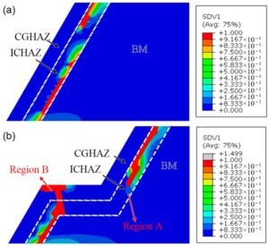
Damage distribution (damage variable ω contours) in two welded joint simulations after creep exposure, from Zhang et al. (2024). Red indicates areas with damage approaching failure (ω ≈ 1). In (a) a conventional V-groove weld, the damage localizes in the HAZ (coarse-grained HAZ, CGHAZ, and intercritical HAZ, ICHAZ, marked by white dashed boundaries) leading to a creep crack in the HAZ. In (b) a stepped groove weld, the damage is more distributed (two regions “A” and “B” are highlighted), deflecting the crack path and resulting in a longer creep life.

The figure above (from an FEA creep study of dissimilar metal welds) vividly shows how damage can concentrate in the HAZ. In (a), with a standard V-groove, the red band (ω ≈ 1) is right along the HAZ – indicating that’s where the creep crack will form. In (b), the weld joint design was modified (stepped groove), and we see two red spots instead of one continuous band; essentially the creep damage was spread out, which in that study improved the overall life. This kind of insight is only obtainable via detailed FEA – it lets engineers experiment with design changes (like groove geometry, material placement, etc.) to mitigate creep damage.

1. Engineering Assessment and Decisions: The final step is using the results to make decisions per FFS guidelines. If the analysis shows adequate remaining life, great – the component can continue service with maybe periodic monitoring. If not, the options might be: reduce operating temperature or stress (if possible), repair or replace the weld, or perform a metallurgical evaluation (sometimes codes call for checking actual creep damage via replica or metallography if predicted life is near end). The analysis could also justify a life extension: for instance, if a crude Level 1 calc said the component is at end-of-life, but your detailed Level 3 FEA shows only 50% damage in reality, you could safely justify running it longer, saving money on unnecessary repairs. Conversely, if the detailed analysis reveals a high damage zone that the crude calc missed, you might prevent a failure by proactively fixing it. This is the value of advanced FFS assessments.

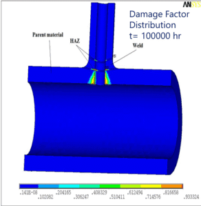
A point worth noting: performing such FEA requires expertise in both welding metallurgy and computational modeling. The calibration of the damage model is critical – you usually adjust the damage model parameters so that the simulation matches known experimental data (like creep rupture times for cross-weld specimens). If not calibrated, the FEA might give garbage results (either overly conservative or non-conservative). When done properly, though, continuum damage FEA has proven quite accurate in replicating real-world creep failures. For example, one study modeled a medium-bore pipe with a welded branch (a complex 3D geometry) and was able to predict creep damage initiation and growth in the HAZ that matched where the actual failures were observed【13†L13-L18**]. That study was part of validating the R5 procedure for high-temperature weld assessments.

(Side note: If you’re wondering about the computational cost – yes, long-term creep FEA can be time-consuming. We often use some tricks, like time scaling (using higher stress or temperature to accelerate creep in the simulation) but have to be careful to still represent the correct damage mechanisms. Modern computers and software optimizations have made it feasible to run even 3D creep damage models in reasonable time, especially for a single weldment.)

Fitness-For-Service (FFS) Level 3 and Advanced Creep Assessments

You may be asking, how do these advanced analyses fit into industry practice? This is where Fitness-For-Service (FFS) standards come into play. FFS is a systematic approach (with codes like API 579-1/ASME FFS-1 or ASME PCC-3, etc.) to evaluate whether equipment with flaws or damage can continue to operate safely. It’s like a structured engineering triage: Level 1 assessments are very conservative and quick (screening criteria), Level 2 are more detailed analytical evaluations, and Level 3 are the most detailed, allowing numerical simulation and custom material modeling.

For creep damage in particular, FFS assessments can be quite involved. API 579-1 Part 10 is dedicated to components operating in the creep regime. A Level 1 creep assessment might simply check if the operating conditions are below the creep threshold for the material or use a very simplified life fraction rule (e.g., compare elapsed time at temperature to a known creep life). If it fails Level 1 (meaning potential creep concerns), you go to Level 2, which might involve calculating creep life based on empirical methods like Larson-Miller Parameter or the Omega method using the provided material data in standards. Level 2 might also involve computing a creep damage factor (the fraction of life used) and seeing if it’s below a certain allowable (often 1.0 or sometimes 0.8 to leave a safety margin).

When those methods are either too conservative or not applicable (for example, in a weld where you don’t have a straightforward way to apply them), Level 3 is invoked. In Level 3, the code essentially says: use all the tools at your disposal (including finite element creep analysis, experimental data, etc.) to perform a rigorous assessment. The goal is to demonstrate fitness-for-service with a higher confidence by reducing unnecessary conservatism. Our entire discussion on continuum damage FEA slots in here as a Level 3 approach. We build a case that, given the simulated damage and life prediction, the component is or isn’t fit for continued use.

To connect with FFS criteria: many codes use a damage summation rule. For example, API 579 recommends that the creep damage fraction (time at temperature divided by allowable time to rupture at that temperature/stress) should not exceed 1.0 (or 0.8 in some cases to include a safety factor). If our advanced analysis shows a certain location reaches 80% damage in 200,000 hours, we might set 200,000 hours as the safe operating life (so that we don’t exceed 100% – actual failure). If there’s also fatigue or other damage, those would be combined per the code rules (e.g., linear damage summation). FFS Level 3 gives the flexibility to use non-standard methods as long as they are sound and well documented. For creep, this could mean using a continuum damage model not explicitly in the code, or doing a full 3D finite element creep simulation, which the code wouldn’t spell out in a step-by-step way but would accept as engineering analysis.

One real-world example of advanced FFS in action: In the refining industry, some pressure vessels showed creep damage and had questionable remaining life by simple calculations. By doing a detailed continuum damage FEA (similar to what we’ve described), engineers were able to show that the creep damage was localized and that the vessel as a whole could operate longer with monitoring. This avoided an expensive premature replacement. On the flip side, another assessment might reveal a severe local creep damage that a plant was not aware of – prompting a targeted weld repair before a failure happens. The power of FFS Level 3 is that it turns “unknown unknowns” into quantifiable predictions, helping teams make informed decisions about run, repair, or retire.

It’s worth mentioning that standards are evolving too. The latest 2021 edition of API 579-1 has updated methodologies for creep. There is also work in progress (for example, a new Annex in API 579 or an upcoming API 586 Recommended Practice) focused on HTHA and creep inspection – indicating that industry recognizes the importance of these damage mechanisms and the need for better guidance. We can expect that advanced techniques, possibly including continuum damage simulations, will become more commonplace and standardized in the future. For now, they are typically the domain of specialists and FFS Level 3 consulting projects.

Conclusion

Creep life assessment of complex and welded components is a challenging but essential task in many industries. Welded joints in high-temperature service can fail insidiously by creep long before a traditional fatigue crack would appear. Through the lens of continuum damage mechanics and aided by finite element analysis, engineers can peel back the mystery and see how damage accumulates inside a weldment – identifying the when, where, and why of potential failures. We discussed how CDM provides a framework to predict tertiary creep and rupture by introducing a damage variable, and how this has been implemented from simple empirical methods like the Omega creep model up to full-blown 3D FE simulations of welded structures. By accounting for the unique behavior of weld metals and HAZ regions, these analyses give far more accurate life predictions than one-size-fits-all formulas.

From a practical standpoint, embracing these advanced techniques can be hugely beneficial. They allow operators to safely extend the life of equipment by avoiding undue conservatism – or conversely, to avoid catastrophic failures by catching underestimated damage. In an FFS Level 3 assessment, using tools like Abaqus or Ansys to perform creep-damage simulation is often the best way to demonstrate that a component is fit (or unfit) for continued service. Yes, it requires specialized expertise, but the investment in a detailed analysis can pay for itself many times over by preventing unplanned downtime or optimizing inspection/maintenance intervals.

At EngineeringDownloads, we have embraced these advanced FFS practices. (Having personally spent years working on creep and weld simulations, I’ve seen how valuable this approach is.) Our team, led by experts like Saman Hosseini, is experienced in continuum creep damage analysis, weld integrity assessments, and FFS Level 3 evaluations. Check out our Example For a Damage Explicit Model on website. We’re passionate about helping industry solve high-temperature materials problems – whether it’s assessing a degraded furnace tube weld or consulting on the design of a new creep-resistant structure. If you’re facing challenges with creep or suspect your equipment may be nearing the end of its life, feel free to reach out for an expert consultation. By combining deep knowledge of metallurgy with cutting-edge simulation techniques, we can chart a safe and economical path forward for your assets.

In the battle against creep damage, knowledge and advanced analysis are our best tools. With these, we can keep critical infrastructure safe, efficient, and reliable for years to come.