Welcome, fellow engineers! Today, we’re diving deep into the Finite Volume Method (FVM) – a cornerstone numerical technique, especially prevalent in Computational Fluid Dynamics (CFD). If you’ve ever wondered how complex fluid flows, heat transfer, or mass transport phenomena are simulated, FVM is likely the engine under the hood. It’s a robust and versatile method that underpins much of the analysis we do in fields ranging from aerospace and automotive design to oil & gas and biomechanics.
Unlike some highly academic treatments, our goal here is to provide a practical, engineer-to-engineer understanding. We’ll strip away the unnecessary mathematical jargon and focus on the core principles, practical implementation, and common challenges you’ll face when applying FVM in your work. Whether you’re working with commercial packages like ANSYS Fluent or OpenFOAM, or even developing your own solvers, grasping FVM fundamentals is crucial for obtaining accurate and reliable simulation results.

Image: A 2D mesh illustrating control volumes in FVM.
What is the Finite Volume Method (FVM)?
At its heart, FVM is a discretization technique used to convert partial differential equations (PDEs) – which describe continuous physical phenomena – into a system of algebraic equations that can be solved numerically on a computer. It’s particularly popular because it naturally conserves quantities like mass, momentum, and energy over discrete control volumes, making it highly suitable for CFD and heat transfer problems.
The Core Idea: Control Volumes
Imagine your complex engineering domain – say, an aircraft wing or a pipeline section. Instead of trying to solve equations at every single point (which is impossible), FVM breaks this domain down into a finite number of non-overlapping, small regions called ‘control volumes’ or ‘cells’.
- Each control volume surrounds a grid point or node.
- The PDEs are then integrated over each control volume.
- This integral formulation naturally ensures conservation of the relevant physical quantity within each control volume.
This conservation property is a significant advantage, as it means that whatever enters a control volume must either leave it or be stored within it, directly reflecting the physical laws of conservation.
Key Principles of FVM
Understanding these principles will give you a solid foundation for interpreting your simulation results.
1. Discretization of the Domain
The first step in any FVM analysis is to divide the continuous physical domain into a finite set of discrete control volumes. This process is known as meshing. The quality and type of mesh significantly impact the accuracy and stability of your solution.
- Structured Meshes: Often composed of quadrilateral (2D) or hexahedral (3D) cells arranged in a regular pattern. Easier to generate and offer good quality, but struggle with complex geometries.
- Unstructured Meshes: Consist of triangular (2D) or tetrahedral (3D) cells, or even polyhedral cells, allowing for greater flexibility in handling complex geometries. They are more challenging to ensure high quality, which is crucial for accuracy.
- Hybrid Meshes: Combine structured and unstructured regions to leverage the strengths of both.
2. Integration over Control Volumes
For each control volume, the governing PDEs (e.g., Navier-Stokes equations for fluid flow) are integrated. This transforms the differential equations into integral equations, which state that the rate of change of a quantity within the control volume plus the net flux of that quantity across the control volume boundaries must equal the generation or consumption of that quantity within the volume.
3. Approximation of Fluxes
The integral equations involve fluxes (e.g., mass flow, heat flux, momentum flux) across the faces of each control volume. Since we only have information at the cell centers (or nodes), we need to approximate these face values. This is where interpolation schemes come into play, which we’ll discuss shortly.
4. Conversion to Algebraic Equations
By approximating the terms in the integrated equations, we arrive at a system of linear algebraic equations for the unknown variables (e.g., velocity, pressure, temperature) at each cell center. This system can then be solved using numerical linear algebra techniques.
Practical Steps in an FVM Simulation
A typical FVM workflow involves several stages, often performed within powerful CAE software packages or using open-source tools.
1. Pre-processing
a. Geometry Definition and Cleanup
- Start with your CAD model (e.g., from CATIA, SolidWorks, AutoCAD).
- Simplify the geometry: remove small features, fillets, or gaps that are irrelevant to the simulation but would complicate meshing.
- Define the computational domain: For external flows, this involves creating an enclosure around your object; for internal flows, it’s the fluid volume itself.
b. Mesh Generation
- Choose an appropriate mesh type (structured, unstructured, polyhedral). Polyhedral meshes are gaining popularity in CFD due to their balance of accuracy and cell count.
- Define mesh density: Areas with high gradients (e.g., boundary layers, recirculation zones) require finer meshes.
- Specify mesh quality criteria: Skewness, aspect ratio, orthogonality. Poor quality meshes are a primary source of simulation errors and divergence. Tools like ANSYS Meshing, HyperMesh, or snappyHexMesh (OpenFOAM) are used here.
c. Boundary Conditions (BCs) and Initial Conditions (ICs)
- Inlets: Specify velocity, pressure, temperature, or mass flow rate.
- Outlets: Specify pressure (e.g., atmospheric), or outflow conditions.
- Walls: Define no-slip (fluid sticks to wall) or slip conditions, and thermal conditions (adiabatic, fixed temperature, heat flux).
- Symmetry/Periodicity: Reduce computational domain for symmetrical or repeating flows.
- Initial Conditions: Provide starting values for all variables. For steady-state problems, these can be rough guesses; for transient problems, they must accurately reflect the starting physical state.
2. Solver Setup
a. Governing Equations and Models
- Select the relevant physical models: Laminar vs. turbulent flow (e.g., k-epsilon, k-omega RANS models), multiphase flow, combustion, heat transfer.
- Define material properties: Density, viscosity, thermal conductivity, specific heat. These can be constant, temperature-dependent, or defined by custom functions (often via user-defined functions, UDFs, in commercial codes or C++ in OpenFOAM).
b. Discretization Schemes
This is where the integral equations are converted into algebraic ones. The choice of scheme affects accuracy, stability, and computational cost.
- First-Order Upwind: Simple, robust, and stable, but highly diffusive (introduces numerical error that smoothes out sharp gradients). Good for initial solutions.
- Second-Order Upwind: More accurate than first-order, less diffusive, but can be less stable. Good for general flows.
- Central Differencing: Second-order accurate, but prone to oscillations and instability for convection-dominated flows if the mesh is not fine enough. Rarely used alone for convective terms.
- QUICK (Quadratic Upstream Interpolation for Convective Kinematics): Third-order accuracy, often used for higher accuracy but can be more complex to implement and potentially less stable.
c. Solution Control
- Solver Type: Coupled (solve all equations simultaneously) or segregated (solve equations sequentially). Segregated is more common in FVM, especially for incompressible flows (e.g., SIMPLE, PISO algorithms).
- Under-Relaxation Factors (URFs): Crucial for stability in iterative solvers. Values between 0 and 1. Too high, and your solution diverges; too low, and it takes too long to converge.
- Convergence Criteria: Define how ‘converged’ your solution needs to be. Typically based on residuals (measure of imbalance in equations), but also monitoring physical quantities (e.g., lift, drag, outlet temperature).
3. Solving
The solver iteratively solves the system of algebraic equations until the convergence criteria are met. This is often the most computationally intensive part.
4. Post-processing
After the solution, we analyze the results to extract meaningful engineering insights.
- Visualizations: Contour plots (pressure, velocity, temperature), vector plots, streamlines, iso-surfaces.
- Quantitative Data: Integrated values (lift, drag, mass flow rate), wall shear stress, heat transfer coefficients, pressure drop.
- Validation: Compare simulation results against experimental data, analytical solutions, or other validated simulations.
FVM vs. Other Discretization Methods
FVM is not the only game in town. Here’s how it stacks up against Finite Element Method (FEM) and Finite Difference Method (FDM).
| Feature | Finite Volume Method (FVM) | Finite Element Method (FEM) | Finite Difference Method (FDM) |
|---|---|---|---|
| Core Principle | Conservation over discrete control volumes (integral form). | Approximation using basis functions over elements (variational/weighted residual form). | Approximation of derivatives at grid points (differential form). |
| Conservation | Inherently conserved, excellent for fluxes. | Can be conserved, but not always inherent. | Not inherently conserved, requires careful implementation. |
| Geometry Handling | Excellent for complex geometries (unstructured meshes). | Excellent for complex geometries (unstructured meshes). | Challenging for complex geometries (typically structured meshes). |
| Primary Application | CFD, Heat Transfer, Mass Transport. | Structural Mechanics (FEA), Solid Mechanics, Electromagnetics. | Simple academic problems, grid-based simulations (e.g., some image processing). |
| Mesh Types | Structured, Unstructured, Polyhedral. | Structured, Unstructured (triangles/quads in 2D, tets/hexes in 3D). | Structured, uniform Cartesian grids. |
| Software Examples | ANSYS Fluent, OpenFOAM, Star-CCM+. | Abaqus, ANSYS Mechanical, MSC Nastran, CalculiX. | Custom codes, MATLAB FDM toolbox. |
Applications of FVM in Engineering
FVM’s versatility makes it indispensable across various engineering disciplines.
- Aerospace Engineering: Simulating airflow over aircraft wings, jet engine performance, understanding hypersonic flows. Tools: Fluent, Star-CCM+.
- Oil & Gas: Pipeline flow analysis, reservoir simulation, offshore platform hydrodynamics, combustion in gas turbines and furnaces. Tools: OpenFOAM, Fluent.
- Automotive Engineering: Aerodynamics of vehicles, engine combustion, thermal management of battery packs, cabin ventilation.
- Biomechanics: Blood flow in arteries, airflow in the respiratory system, drug delivery.
- Civil Engineering: Wind loads on buildings, pollutant dispersion, water flow in rivers and pipes.
- Process Engineering: Mixer design, chemical reactor optimization, heat exchanger performance.
Practical Workflow: Mastering Your FVM Simulations
To consistently achieve accurate FVM results, follow a structured workflow, especially focusing on critical aspects of mesh, boundary conditions, and solver settings.
Step-by-Step Simulation Checklist:
- Define Objectives: What specific outputs do you need? (e.g., drag coefficient, temperature distribution, pressure drop).
- Simplify Geometry: Use CAD tools (e.g., CATIA, SolidWorks) to create a clean, watertight model suitable for meshing.
- Mesh Generation: Create a mesh. Use local refinements in critical regions (e.g., near walls, shear layers). Ensure cell quality metrics are within acceptable ranges. For example, a maximum skewness of 0.85 is often a good target.
- Apply Boundary Conditions: Accurately represent physical conditions. Double-check units and directions.
- Select Physical Models: Choose appropriate turbulence models (if applicable), radiation models, multiphase models, etc., based on flow regime and physics.
- Choose Discretization Schemes: Start with first-order for stability, then switch to second-order or higher once a stable solution is achieved.
- Set Solver Controls: Adjust under-relaxation factors carefully. Monitor residuals and key physical quantities for convergence.
- Run Simulation: Use sufficient iterations for steady-state or timesteps for transient problems.
- Post-Process Results: Visualize, extract data, compare with objectives.
- Verification & Validation: Crucial for confidence in results.
Verification & Sanity Checks for FVM Simulations
Never blindly trust your simulation results. Always perform verification and validation steps to ensure accuracy and reliability.
1. Mesh Independence Study
This is arguably the most critical check. Run your simulation with progressively finer meshes and observe if your key results (e.g., drag, pressure drop, heat transfer rate) change significantly. Once these quantities stop changing beyond a certain tolerance (e.g., 1-2%), your solution is considered ‘mesh independent’. If you’re working with Python or MATLAB, you can automate this process by scripting mesh generation and result extraction.
2. Boundary Condition Sensitivity
How sensitive are your results to small changes in boundary conditions? For example, if you’re simulating a valve, how does a slight variation in inlet pressure affect the flow rate? This helps understand the robustness of your model and the physical system.
3. Convergence Criteria
Ensure that not only the residual values drop below a target (e.g., 1e-4 or 1e-5), but also that the monitored physical quantities reach a steady value. Oscillating residuals or physical quantities indicate a non-converged or unsteady solution. For transient simulations, ensure your time step is small enough to capture the relevant phenomena.
4. Physical Plausibility
Do the results make sense physically? Are velocities unrealistically high or low? Are temperatures within expected ranges? Is there mass conserved? (e.g., total mass flow in = total mass flow out). Use engineering judgment and back-of-the-envelope calculations.
5. Code and Model Validation
Whenever possible, compare your simulation results against:
- Experimental Data: The gold standard for validation.
- Analytical Solutions: For simplified cases, these provide exact benchmarks.
- Published Literature/Benchmarks: Compare against validated results from similar studies.
Common Pitfalls and Troubleshooting in FVM
Even experienced engineers encounter issues. Here’s how to navigate common FVM challenges.
1. Divergence Issues
Your simulation fails to converge, or worse, gives ‘NaN’ (Not a Number) errors.
- Troubleshooting:
- Poor Mesh Quality: Check skewness, aspect ratio, orthogonality. Remesh problematic areas.
- Aggressive Under-Relaxation Factors: Reduce URFs, especially for pressure, momentum, and turbulence.
- Incorrect Boundary Conditions: Double-check units, values, and location. Ensure consistency (e.g., mass flow rate at inlet matches a reasonable outlet pressure).
- Bad Initial Conditions: Provide a more physically realistic start for complex flows, or run a short simulation with first-order schemes to get a better initial guess.
- Unsuitable Discretization Scheme: Start with first-order schemes for all variables to gain stability, then gradually introduce higher-order schemes.
- Physical Instabilities: Is your flow inherently unsteady? Consider a transient simulation.
2. Inaccurate Results
Your simulation converges, but the numbers don’t seem right or don’t match reality.
- Troubleshooting:
- Insufficient Mesh Resolution: Your mesh might be too coarse in critical regions. Perform a mesh independence study.
- Wrong Physical Models: Is your turbulence model appropriate for the flow? Are material properties correct?
- Boundary Condition Errors: Even subtle errors can lead to large discrepancies.
- Convergence Not Fully Achieved: Check if key physical quantities have truly converged, not just residuals.
- Numerical Diffusion: First-order schemes can artificially smooth out sharp gradients. Switch to second-order or higher once the solution stabilizes.
3. Long Simulation Times
Your simulation takes forever to run.
- Troubleshooting:
- Overly Fine Mesh: While accuracy is good, an excessively fine mesh, especially in regions of low interest, will dramatically increase computation time. Balance accuracy with computational cost.
- Small Timesteps: For transient simulations, if your timestep is too small, it will take many steps to reach the desired physical time. Use adaptive timestepping if available.
- Poor Initial Conditions: A bad IC means the solver spends a lot of time finding the solution.
- Aggressive Under-Relaxation Factors: While too low URFs can stabilize divergence, they can also slow down convergence. Find the sweet spot.
- Inefficient Solver Settings: Ensure you are utilizing available parallel processing capabilities and efficient linear solvers.
Leveraging Tools & Automation for FVM
Modern engineering demands efficiency. Tools and automation can significantly streamline your FVM workflows.
Commercial Software
- ANSYS Fluent/CFX: Industry-standard for complex CFD simulations, offering comprehensive models and user-friendly interfaces.
- Siemens Star-CCM+: Another powerful, integrated CFD solution known for its meshing capabilities and multi-physics approach.
- Abaqus (CFD Module): While primarily an FEA tool, it has capabilities for some CFD problems, especially coupled with structural analysis.
Open-Source Alternatives
- OpenFOAM: A free, open-source C++ toolbox for developing custom CFD solvers and utilities. Requires programming knowledge but offers immense flexibility. It’s widely used in academia and increasingly in industry for specialized applications.
- SU2: An open-source suite for CFD and design optimization, developed at Stanford University.
Python & MATLAB for Automation
Don’t underestimate the power of scripting for pre- and post-processing:
- Python: Libraries like NumPy, SciPy, Matplotlib, and Paraview (via
pvpython) are invaluable for generating complex boundary conditions, automating mesh parameter studies, extracting specific data from large result files, and creating custom plots. Many commercial codes offer Python APIs for scripting. - MATLAB: Excellent for rapid prototyping, data analysis, and visualization. Useful for developing simplified models, processing experimental data for validation, or creating custom post-processing scripts.
If you’re looking to enhance your automation skills or need bespoke scripts for your FVM projects, explore the downloadable templates, projects, and custom scripting services offered by EngineeringDownloads.com. Our experts can also provide tailored online consultancy and tutoring to help you master these techniques.
Concluding Thoughts
The Finite Volume Method is a powerful and essential tool in the modern engineer’s arsenal, particularly for simulating fluid flow and related phenomena. By understanding its fundamental principles, meticulously following practical workflows, and diligently performing verification and validation, you can unlock its full potential to solve complex engineering challenges. Keep learning, keep questioning your results, and leverage the fantastic array of tools and resources available to you.
Further Reading
For a deeper dive into the theoretical aspects and detailed equations of FVM, consider consulting authoritative resources suchp as the CFD-Online Wiki on the Finite Volume Method.