Welcome, fellow engineers! Today, we’re diving deep into the Finite Element Method (FEM) – a cornerstone of modern engineering analysis. Whether you’re designing aerospace components, analyzing structural integrity in oil & gas, or optimizing medical implants, FEM, and its application in Finite Element Analysis (FEA), is an indispensable tool. This isn’t an academic lecture; it’s a practical, engineer-to-engineer guide to understanding, applying, and mastering FEM for real-world problems.

Image illustrating a finite element mesh on a plate with a hole.
What is the Finite Element Method (FEM)?
At its heart, FEM is a numerical technique for finding approximate solutions to boundary value problems for partial differential equations (PDEs). In engineering, this means solving complex problems in fields like structural mechanics, heat transfer, fluid flow, and electromagnetism that would be impossible or impractical to solve analytically.
Think of it this way: you have a complex engineering problem – perhaps predicting stress in a turbine blade or temperature distribution in a heat exchanger. FEM breaks down this complex structure into a large number of smaller, simpler, interconnected components called ‘finite elements’. Within each element, the governing equations are approximated, and then these approximations are assembled to represent the entire system. This ‘divide and conquer’ approach allows us to tackle highly intricate geometries and loading conditions.
Why FEM is Crucial for Modern Engineers
- Design Optimization: Iterate designs rapidly to improve performance, reduce weight, or cut costs without costly physical prototypes.
- Failure Prediction: Identify potential failure points, assess structural integrity (vital for FFS Level 3 assessments), and understand fatigue life.
- Safety & Compliance: Ensure designs meet industry standards and safety regulations, particularly in critical sectors like aerospace and oil & gas.
- Understanding Complex Behavior: Simulate non-linear materials, large deformations, contact, and multi-physics phenomena.
The Core Idea: Discretization and Approximation
The entire FEM philosophy revolves around two fundamental concepts:
1. Discretization: Breaking Down the Problem
This is where your complex component is divided into a mesh of finite elements. Imagine a 3D object; we ‘discretize’ it into thousands or millions of tiny, simple shapes like tetrahedrons or hexahedrons. For a 2D plate, we might use triangles or quadrilaterals. Each corner or intersection point of these elements is called a ‘node’.
Element Types and Their Applications
- 1D Elements (Bars, Beams, Trusses): Ideal for slender structures where behavior is predominantly axial or bending. Commonly used in truss analyses or framework structures.
- 2D Elements (Shells, Plates, Membranes): Suitable for thin-walled structures where one dimension is significantly smaller than the others (e.g., aircraft fuselage panels, pressure vessel walls).
- 3D Elements (Solids – Tetrahedrons, Hexahedrons): For chunky, volumetric components where stress and strain vary significantly in all three dimensions (e.g., engine blocks, turbine disks, complex mechanical parts).
The choice of element type is critical and depends on the geometry, the physics of the problem, and the desired accuracy versus computational cost. Modern CAD-CAE workflows integrate seamlessly, allowing you to import your geometry from tools like CATIA and prepare it for meshing.
2. Approximation: Solving Locally
Within each finite element, we assume a simple mathematical function (often a polynomial) to approximate the unknown field variable (e.g., displacement, temperature, pressure). These are called ‘shape functions’ or ‘interpolation functions’. These functions relate the unknown values within the element to the known values at its nodes.
By using these approximations for each element, we convert a complex continuous problem into a system of algebraic equations. When these elemental equations are assembled for the entire structure, we get a global system of equations that can be solved numerically using powerful computational methods.
Key Concepts in FEM: The Engineer’s Toolkit
Governing Equations & The Weak Form
Every physical phenomenon is governed by a set of differential equations. In FEM, we often transform these ‘strong form’ differential equations into a ‘weak form’ (e.g., using the principle of virtual work for structural mechanics or Galerkin’s method). This transformation makes the problem easier to solve numerically and allows for less stringent continuity requirements on the approximation functions.
Don’t get bogged down in the heavy math here; the key takeaway is that the weak form is what the FEA software actually solves. It ensures that, on average, the equations are satisfied across the element and the entire domain.
Element and Global Stiffness Matrices
For structural problems, each element has an ‘element stiffness matrix’ ([k]) that relates the forces applied to an element’s nodes to the resulting displacements. These individual element matrices are then ‘assembled’ into a much larger ‘global stiffness matrix’ ([K]) for the entire structure. This global matrix, along with the global nodal displacement vector ({u}) and global nodal force vector ({F}), forms the core FEM equation:
[K]{u} = {F}
Solving this system of equations for {u} gives us the nodal displacements, which are the fundamental unknowns we are seeking.
Boundary Conditions (BCs) and Loads: Defining Reality
Correctly applying boundary conditions and loads is arguably the most critical step in any FEA simulation. These define how your structure interacts with its environment.
Types of Boundary Conditions:
- Displacement BCs (Essential/Dirichlet): You directly specify the displacement at a node. Examples: fixing a part in space (
u=0, v=0, w=0), allowing movement in only one direction. - Force/Traction BCs (Natural/Neumann): You specify the force or pressure acting on a surface or node. Examples: a point load, distributed pressure from fluid, gravity.
Tips for Applying BCs:
- Realism: Ensure BCs accurately represent how the component is supported and loaded in reality. Over-constraining can lead to artificially high stresses. Under-constraining leads to rigid body motion (instability).
- Symmetry: Utilize symmetry planes to reduce model size and computational time, but apply appropriate symmetry BCs (e.g., no displacement normal to the plane, no rotation about axes in the plane).
- Contact: For assemblies, define contact interactions carefully. This can significantly impact stress distribution.
A Practical FEM Workflow: From CAD to Insights
Here’s a step-by-step guide to conducting a robust FEA simulation:
1. Problem Definition & Objectives
- Clearly define what you want to achieve: stress distribution, displacement, natural frequencies, heat flux, etc.
- Identify the critical regions and potential failure modes.
- Gather all relevant data: geometry, material properties, loading scenarios, environmental conditions.
2. CAD Model Preparation
- Import your CAD model (e.g., from SolidWorks, CATIA, Inventor).
- Simplify Geometry: Remove small features (fillets, chamfers, small holes) that don’t significantly impact global behavior but drastically increase mesh complexity. This is crucial for efficient meshing in tools like Abaqus or ANSYS Mechanical.
- Mid-Surfacing/Shelling: For thin-walled structures, extract mid-surfaces to create 2D shell models, which are computationally much cheaper than 3D solid models.
3. Material Properties & Constitutive Models
- Define accurate material properties: Young’s Modulus, Poisson’s Ratio, Density, Yield Strength, Thermal Conductivity, etc.
- Choose appropriate constitutive models: Linear elastic, elastoplastic, hyperelastic, viscoelastic, creep, etc., depending on the material and expected behavior.
4. Meshing Strategy
- Element Choice: Select appropriate element types (1D, 2D, 3D) and order (linear vs. quadratic). Quadratic elements generally provide better accuracy with fewer elements for bending-dominated problems.
- Mesh Density: Refine the mesh in areas of high stress gradients or critical features (stress concentrations). Use coarser meshes in less critical areas to save computational resources.
- Mesh Quality: Pay attention to aspect ratio, skewness, and Jacobian for 3D elements. Poor quality elements can lead to inaccurate or failed solutions.
5. Applying Loads & Boundary Conditions
- As discussed, apply forces, pressures, displacements, temperatures, etc., precisely where they occur in the real world.
- Ensure all rigid body motions are constrained, but avoid over-constraining.
6. Solving the System
- Select the appropriate analysis type (static, dynamic, thermal, buckling, etc.).
- Configure solver settings (e.g., time steps for non-linear problems, convergence criteria).
- Submit the job to the solver (e.g., Abaqus/Standard, ANSYS Mechanical APDL, MSC Nastran).
7. Post-Processing & Interpretation
- Visualize results: Stress contours, displacement plots, strain fields, temperature maps.
- Identify maximum/minimum values, critical locations.
- Compare results against yield strength, buckling limits, or other design criteria.
- Generate reports and animations.
Common Applications of FEM in Engineering
- Structural Engineering: Analyzing buildings, bridges, and infrastructure for stress, deflection, vibration, and seismic response.
- Aerospace: Design and analysis of aircraft structures, engine components, and spacecraft for extreme loads, fatigue, and aeroelasticity. Tools like Abaqus and ANSYS are heavily used.
- Oil & Gas: Integrity assessment of pipelines, offshore platforms, pressure vessels, and drilling equipment, often involving FFS Level 3 assessments and multi-physics simulations.
- Biomechanics: Modeling medical implants, prosthetic devices, and human tissue response under various loads.
- Automotive: Crashworthiness, NVH (Noise, Vibration, Harshness), powertrain design, and component optimization using tools like ADAMS for multibody dynamics, often integrated with FEA.
- Thermal Analysis: Predicting temperature distributions, heat flux, and thermal stresses in electronic components, engines, and industrial processes.
- Fluid-Structure Interaction (FSI): Coupling FEA with CFD (e.g., ANSYS Fluent/CFX or OpenFOAM) to simulate problems where fluid flow affects structural deformation and vice-versa (e.g., wind turbine blades, heart valves).
Verification & Sanity Checks: Trusting Your Results
Never take FEA results at face value. A sophisticated simulation program can still give you garbage if the inputs are flawed. Here’s your checklist:
- Convergence Studies: Perform a mesh convergence study. Does refining the mesh significantly change your critical results (e.g., max stress, displacement)? If so, your mesh might be too coarse. Also, check solution convergence for non-linear problems.
- Hand Calculations/Analytical Solutions: For simplified cases or regions, can you perform a quick hand calculation (e.g., beam bending, simple tension)? Does your FEA result compare reasonably?
- Symmetry Checks: If you used symmetry, ensure the results along the symmetry plane make physical sense (e.g., no displacement perpendicular to a symmetry plane for stress analysis).
- Units Consistency: Double-check all units! It’s a common source of error. Use a consistent system (e.g., N, mm, MPa, or lbf, in, psi).
- Deformation Plots: Animate the deformation. Does it look physically plausible? Are there any unexpected distortions or ‘hourglassing’ effects?
- Reaction Forces: Sum the reaction forces at constrained boundaries. Do they balance the applied loads? This is a fundamental check.
- Energy Balance: For dynamic or non-linear analyses, check the energy balance if your solver provides it. Ensure internal energy equals external work done.
- Sensitivity Analysis: How sensitive are your results to small changes in material properties, loads, or BCs? This helps understand the robustness of your design.
Choosing the Right FEA Software
The market offers a range of powerful FEA software packages, each with its strengths. Your choice will depend on your industry, the complexity of your problems, available budget, and desired features.
| Software | Key Strengths | Common Applications |
|---|---|---|
| Abaqus (Dassault Systèmes) | Advanced non-linear, multi-physics, explicit dynamics, material modeling. | Aerospace, Automotive, Research, Biomechanics (complex materials). |
| ANSYS Mechanical | Comprehensive suite, broad capabilities (structural, thermal, FSI), user-friendly GUI. | General engineering, structural analysis, product design, oil & gas. |
| MSC Nastran | Strong legacy in linear structural analysis, vibrations, acoustics. | Aerospace, Automotive (NVH, linear statics). |
| SimScale / Onshape Sim. | Cloud-native, collaborative, good for accessible FEA/CFD. | SMBs, educational, rapid prototyping. |
| Open Source (e.g., Code_Aster, CalculiX) | Cost-effective, highly customizable, community-driven. | Research, specialized applications, users with coding expertise. |
Many of these tools also integrate with CAD software (like CATIA for Abaqus) for a streamlined CAD-CAE workflow.
Automation in FEA: Python & MATLAB for Efficiency
As an engineer, you know efficiency is key. Python and MATLAB are invaluable for automating repetitive FEA tasks and extending software capabilities:
- Scripting Pre- & Post-Processing: Automate model setup (geometry creation, material assignment, meshing strategies), load application, and results extraction. Many commercial FEA packages (Abaqus, ANSYS) have Python APIs.
- Parametric Studies & Optimization: Run hundreds or thousands of simulations by varying design parameters systematically. This is crucial for design exploration and optimization.
- Custom Post-Processing: Develop custom scripts to process and visualize results in unique ways, or to integrate FEA data with other analyses.
- Integration: Connect FEA tools with other analysis software or data management systems.
Explore our library of downloadable templates, projects, and scripts for FEA automation on EngineeringDownloads.com. We also offer online tutoring and consultancy to help you master these powerful techniques.
Common Pitfalls & How to Avoid Them
- Poor Mesh Quality: Leading to inaccurate results or solver convergence issues. Tip: Prioritize element quality over quantity. Use mesh controls, appropriate element types, and check quality metrics.
- Incorrect Boundary Conditions: Over-constraining (too stiff) or under-constraining (rigid body motion). Tip: Always perform simple checks (reaction forces, deformation plots) and understand how your real component is supported.
- Material Model Mismatch: Using linear elastic when plastic deformation or non-linear material behavior is significant. Tip: Understand the material’s behavior under expected loads. Start simple, then add complexity if needed.
- Ignoring Non-Linearities: Neglecting large deformation, contact, or material non-linearity when they are dominant. Tip: Always consider if non-linear effects are relevant. If displacements are large, or contact is significant, linear analysis will be inaccurate.
- Over-Reliance on ‘Black Box’ Results: Not understanding the underlying theory or the solver’s assumptions. Tip: Always question your results, perform sanity checks, and develop a strong theoretical understanding of FEM.
- Unit Inconsistency: Mixing unit systems within the same model. Tip: Adopt a consistent unit system from the start and stick to it.
The Future of FEM
FEM is continuously evolving. We’re seeing exciting developments in:
- AI/Machine Learning Integration: For accelerating simulations, optimizing designs, and predicting material properties.
- Cloud Computing: Making high-performance computing more accessible for complex analyses.
- Real-Time Simulation: Pushing the boundaries towards real-time predictive capabilities for design and operational insights.
- Additive Manufacturing: Simulation tools are crucial for optimizing designs for 3D printing, predicting distortions, and validating performance of complex geometries.
Further Reading
For a deeper dive into the mathematical foundations, consider exploring resources like MIT OpenCourseware on Finite Element Analysis.
Conclusion
FEM is more than just software; it’s a powerful methodology that empowers engineers to innovate, optimize, and validate designs across virtually every industry. By grasping the fundamentals – discretization, approximation, meshing, and careful application of BCs – and integrating robust verification practices, you can leverage FEA to its full potential. Stay curious, keep learning, and remember that sound engineering judgment is always your most valuable tool.