Mastering Creep Analysis: A Practical Guide for Engineers

Creep Analysis
Hosseini Saman
March 11, 2026
18 Minute

When designing components for demanding environments, especially those involving sustained loads at elevated temperatures, engineers face a critical challenge: creep. Creep is the time-dependent deformation of a material under constant stress, a phenomenon that can lead to catastrophic failure if not properly accounted for. This comprehensive guide will equip you with the knowledge and practical insights needed to confidently approach creep analysis in your engineering projects.

Creep analysis is essential across various industries, from aerospace and power generation to oil & gas and biomechanics. Ignoring creep can compromise structural integrity, leading to costly downtime, safety hazards, and premature equipment failure. Let’s dive into understanding this fascinating yet formidable material behavior.

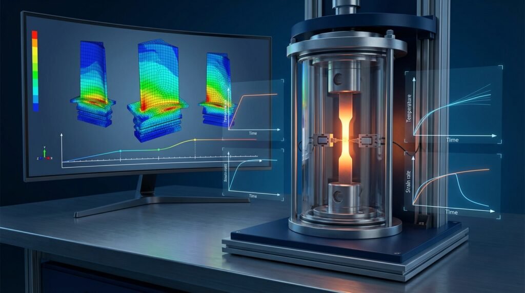
Image: Typical creep curve illustrating the three stages of deformation under constant load. Source: Wikimedia Commons.

Understanding Creep: The Time-Dependent Challenge

Creep is not an instantaneous failure but a gradual process. Imagine a metal beam supporting a load in a high-temperature furnace. Over time, even if the load is well below the material’s yield strength, the beam will slowly elongate or sag. This is creep in action.

What is Creep? A Fundamental Overview

Definition: Creep is plastic deformation that occurs over a prolonged period under constant mechanical stress, typically at temperatures above approximately 0.3 to 0.4 times the material’s absolute melting temperature (T_m).
Key Conditions: Sustained stress and elevated temperature are the primary drivers. The higher the temperature and stress, the faster the creep rate.
Microscopic Mechanisms: At a micro-structural level, creep involves atomic diffusion, dislocation climb, grain boundary sliding, and vacancy movement within the material.
Implications: Creep can lead to excessive deformation, stress redistribution, eventual fracture (creep rupture), and overall loss of dimensional stability.

Why Creep Analysis Matters in Engineering Design

Failing to consider creep during design can have severe consequences. Here’s why it’s a critical aspect of structural integrity and design validation:

Safety: In industries like aerospace (jet engine components), power generation (boiler tubes, steam pipes), and oil & gas (high-temperature pipelines, pressure vessels), creep failure can be catastrophic, leading to explosions, leaks, or collapse.
Reliability: Components designed against creep will have a longer operational life, reducing maintenance costs and increasing system uptime.
Economic Impact: Premature component replacement due to creep damage is expensive. Accurate creep analysis helps optimize material usage and predict service life.
Compliance: Many industry standards (e.g., API 579-1/ASME FFS-1 Level 3 for Fitness-For-Service) mandate creep assessment for high-temperature equipment.

The Three Stages of Creep Deformation

A typical creep curve, plotting strain versus time, reveals three distinct stages:

Primary (Transient) Creep: An initial stage where the creep rate decreases with time. This is due to work hardening, as the material resists further deformation.
Secondary (Steady-State) Creep: The creep rate becomes nearly constant. Here, the hardening and recovery processes within the material are balanced. This stage is often used to define the material’s minimum creep rate.
Tertiary (Accelerated) Creep: The creep rate accelerates rapidly, leading to necking, void formation, and eventually fracture (creep rupture). This stage is often initiated by microstructural changes, such as grain boundary separation or severe damage accumulation.

Let’s summarize these stages in a helpful table:

Creep Stage	Characteristics	Microscopic Behavior	Design Relevance
Primary (Transient)	Creep rate decreases over time	Work hardening, dislocation interaction	Initial deformation, hardening phase
Secondary (Steady-State)	Constant (minimum) creep rate	Balance of hardening and recovery	Predicting long-term deformation, rupture life
Tertiary (Accelerated)	Creep rate accelerates to failure	Void growth, necking, micro-cracking	Critical failure prediction, end-of-life

Key Parameters and Material Behavior in Creep

Understanding the factors that influence creep and how materials are characterized is fundamental to effective creep analysis.

Factors Influencing Creep Performance

Temperature: The most significant factor. Even small temperature increases can dramatically accelerate creep rates.
Stress Level: Higher applied stress leads to faster creep deformation and shorter rupture times.
Time: Creep is inherently a time-dependent phenomenon. Analysis must consider the full service life of the component.
Material Microstructure: Grain size, presence of precipitates, alloying elements, and heat treatment significantly impact a material’s creep resistance. For instance, coarse-grained materials often exhibit better creep resistance.
Environment: Corrosive environments can interact with creep mechanisms, often accelerating degradation (cree-corrosion interaction).

Common Creep-Resistant Materials

Materials selected for high-temperature applications are specifically engineered to resist creep. These include:

Nickel-Based Superalloys: Used extensively in jet engines and gas turbines due to their excellent strength and creep resistance at extreme temperatures.
Stainless Steels (Austenitic): Alloys like 304H and 316H are common in power plants and process industries for their balance of corrosion resistance and moderate creep strength.
High-Temperature Steels: Chromium-molybdenum (Cr-Mo) steels are widely used in pressure vessels and piping for their good creep resistance up to ~550°C.
Ceramics and Composites: Advanced ceramics (e.g., silicon nitride) and ceramic matrix composites (CMCs) are being developed for even higher temperature applications where metals fail.

Creep Data and Constitutive Models

Accurate creep analysis relies heavily on reliable material data. This data is typically obtained from extensive experimental testing (e.g., uniaxial tensile creep tests, stress rupture tests).

Stress-Rupture Curves: Plot time to rupture against applied stress at various temperatures. These are crucial for predicting component lifetime.
Larson-Miller Parameter (LMP): A common time-temperature parameter used to correlate stress rupture data from different temperatures and extrapolate to longer times or different temperatures.
Creep Strain Data: Strain-time curves at different stress and temperature levels provide the basis for constitutive creep models.

Popular Creep Models for Simulation

Constitutive models describe how materials behave under creep conditions and are essential inputs for FEA software:

Norton’s Power Law: A widely used empirical model for secondary creep, relating creep strain rate to stress and temperature.
dε/dt = A * σ^n * exp(-Q/RT) where A, n, Q are material constants.
Dorn’s Law: Similar to Norton’s, but often used to emphasize the temperature dependence through an activation energy term.
Viscoplastic Models: More complex models (e.g., Chaboche, Anand, Bodner-Partom) capture primary and tertiary creep behavior, stress relaxation, and cyclic loading effects.

Performing Creep Analysis with FEA (Finite Element Analysis)

FEA is an indispensable tool for creep analysis, especially for complex geometries, non-uniform stress states, and thermal gradients typical in real-world components.

When to Use FEA for Creep Analysis

When analytical solutions are insufficient due to geometric complexity.
To predict stress redistribution over time due to creep.
To evaluate component life under combined mechanical and thermal loading.
For Fitness-For-Service (FFS) assessments, particularly API 579-1/ASME FFS-1 Level 3 evaluations.
To optimize designs for creep resistance and extend service life.

Practical Workflow for Creep Analysis in FEA

Whether you’re using Abaqus, ANSYS Mechanical, MSC Nastran, or other FEA packages, a structured approach is key.

Step 1: Define Your Problem and Scope

Identify Operating Conditions: What are the maximum and minimum operating temperatures, pressures, and other mechanical loads?
Service Life: What is the target service duration for the component (e.g., 20 years, 100,000 hours)?
Failure Criteria: What constitutes failure? Excessive deformation (strain limit), creep rupture (time to rupture), or stress relaxation?
Material Selection: Confirm the specific material grade and its known creep characteristics.

Step 2: Material Data Acquisition and Modeling

Gather Data: Obtain creep data (creep strain vs. time, stress-rupture data) from material handbooks (e.g., ASME B&PV Code, API RP 579-1), internal company tests, or academic sources.
Fit Creep Laws: Input this data into your FEA software to define the material’s creep behavior. Most commercial codes like Abaqus and ANSYS Mechanical offer various built-in creep models (e.g., Norton, user-defined subroutines for more complex viscoplasticity).
Temperature Dependence: Ensure your material model correctly captures the strong temperature dependency of creep.

Step 3: Geometry and Meshing Considerations

Model Preparation: Simplify the geometry as much as possible without losing critical features.
Element Type: Use elements appropriate for creep analysis. Often, reduced integration elements (e.g., C3D8R in Abaqus, SOLID186 in ANSYS) are preferred to avoid volumetric locking, especially with large deformations.
Mesh Density: Refine the mesh in high-stress gradient regions (e.g., stress concentrations, fillets, welds) where creep deformation will be most pronounced. A coarser mesh elsewhere can save computational cost.

Step 4: Boundary Conditions and Loading

Mechanical Boundary Conditions (BCs): Apply all relevant mechanical loads (pressure, forces, moments) and displacement constraints to prevent rigid body motion.
Thermal Boundary Conditions: Define the temperature distribution throughout the component. This can be a uniform temperature, or a complex transient thermal profile from a CFD analysis (e.g., using ANSYS Fluent/CFX or OpenFOAM, then mapping results to a structural model).
Load Application: Loads are typically applied in steps: first, instantaneous elastic-plastic deformation, then the time-dependent creep analysis.

Step 5: Solver Setup and Time Increment Control

Analysis Type: Select a non-linear static or transient structural analysis with creep enabled.
Time Stepping: This is crucial. Creep simulations involve integrating time-dependent equations.
- Initial Time Step: Start with a small time increment.
- Automatic Time Stepping: Most FEA solvers have automatic time stepping algorithms that adjust the increment size based on convergence criteria and creep strain rate changes. This helps manage computational expense while maintaining accuracy.
Convergence Criteria: Set appropriate convergence tolerances for force/moment and displacement.
Solver Type: Implicit solvers are generally used for creep analysis due to their stability with large time steps, though explicit solvers can be used for highly non-linear or dynamic problems involving creep.

Step 6: Post-Processing and Interpretation of Results

Creep Strain: Analyze total creep strain and creep strain rate distributions. Identify areas with excessive deformation.
Stress Redistribution: Observe how stresses redistribute over time. Stress concentrations often relax, while stresses in other areas might increase.
Creep Damage: Many models incorporate a creep damage parameter, which accumulates over time, indicating proximity to rupture.
Displacement and Distortion: Check overall component deformation and compare it against design limits.
Time to Rupture: Estimate the component’s remaining life based on creep rupture criteria.

If you’re tackling complex creep models or need to speed up your simulations, EngineeringDownloads offers affordable HPC rental services and expert project consultancy to optimize your CAE workflows.

Verification and Sanity Checks in Creep FEA

Trusting your simulation results is paramount. Always perform thorough verification and sanity checks.

Mesh Convergence Study: Run the simulation with progressively finer meshes. Ensure that key results (e.g., maximum stress, strain, displacement) do not change significantly with further mesh refinement.
Boundary Condition (BC) Validation: Carefully review applied loads and constraints. Do they accurately represent the real-world conditions? Is the model over-constrained or under-constrained?
Initial Elastic-Plastic Response: Before creep dominates, the initial response should match an elastic or elastic-plastic analysis without creep.
Steady-State Check: In the secondary creep regime, observe if the creep strain rate stabilizes, indicating the steady-state.
Energy Balance: For transient analyses, monitor energy balances to ensure numerical stability.
Sensitivity Analysis: Evaluate the impact of variations in material properties, temperature, or load on the results. This helps identify critical parameters.
Comparison with Analytical Solutions/Hand Calculations: For simplified cases (e.g., a simple beam), compare FEA results with theoretical predictions to build confidence.
Physical Intuition: Do the results make sense physically? Are deformation patterns and stress distributions as expected?

Common Challenges and Pitfalls in Creep Analysis

Creep analysis can be tricky. Be aware of these common hurdles:

Inaccurate Material Data: The quality of your material model directly dictates the accuracy of your results. Poor experimental data or inappropriate creep constitutive equations are major sources of error.
Meshing and Element Type Issues: Using a mesh that’s too coarse in critical regions or inappropriate element types can lead to inaccurate stress/strain predictions or convergence difficulties.
Boundary Condition Mismatches: Incorrectly applied loads or constraints can drastically alter the stress state and creep response. Ensure your BCs reflect actual service conditions.
Computational Expense: Creep simulations are inherently time-consuming due to the iterative, time-dependent nature of the problem. Long service lives translate to very long simulation times.
Interpreting Complex Results: The non-linear and time-dependent nature of creep can produce complex stress and strain redistribution patterns that require careful interpretation.
Extrapolation of Creep Data: Often, available creep data does not cover the full service life or temperature range. Extrapolating data too far can introduce significant uncertainties.

Troubleshooting Your Creep Simulation

Encountering issues? Here’s a troubleshooting guide:

Checklist for Simulation Success

Material Model Review: Double-check the creep law parameters. Are they for the correct temperature range?
Time Increment Control: If the simulation fails to converge or takes too long, adjust automatic time stepping parameters. Start with very small initial steps.
Non-Linear Convergence: Ensure that the maximum number of iterations is sufficient and that Newton-Raphson settings are appropriate for non-linear behavior.
Contact Definitions: If contact is present, ensure correct contact behavior (e.g., frictionless, rough, cohesive) and proper contact stabilization.
Debug Output: Review solver message files for warnings or error messages that can pinpoint the problem.
Simplify and Test: If a complex model fails, simplify the geometry or loading. Get a simpler model to run, then gradually reintroduce complexity.

Tips for Optimizing Creep Analysis Performance

Sub-modeling: Run a coarse global model, then apply displacements/forces to a refined sub-model of a critical region to save computational time.
Parallel Processing (HPC): Leverage multi-core processors or HPC clusters to distribute calculations and significantly reduce solution time.
Smart Meshing: Use adaptive meshing techniques where the mesh refines automatically in high-gradient regions as the solution progresses.
Material Model Simplification: If a simpler creep law (e.g., Norton’s) yields acceptable accuracy for your problem, avoid unnecessarily complex viscoplastic models.

Leveraging Scripting for Automation (Python & MATLAB)

For repetitive tasks, parameter studies, or custom post-processing, scripting can be a game-changer:

Input File Generation: Use Python or MATLAB to generate parameterized input files for Abaqus or ANSYS, allowing for rapid iteration and design optimization.
Batch Processing: Automate running multiple simulations with varying parameters (e.g., temperature, stress levels).
Custom Post-Processing: Extract specific results, perform custom calculations (e.g., remaining life estimation using Monkman-Grant relation), and generate custom plots or reports.
Data Management: Manage large datasets from multiple simulations efficiently.

Creep Analysis in Specific Engineering Contexts

Creep analysis plays a vital role in ensuring the long-term integrity of structures across various sectors.

Oil & Gas Industry

High-temperature processing units, such as furnaces, reformers, and crude distillation units, operate at elevated temperatures for decades. Creep analysis is critical for:

Pressure Vessels and Piping: Assessing the remaining life and integrity of components under internal pressure and high temperatures. This is a key part of Fitness-For-Service (FFS) assessments, often following API 579-1/ASME FFS-1 Level 3 procedures.
Support Structures: Evaluating the long-term stability of supports for hot pipelines and equipment, which can creep and sag over time.
Material Selection: Guiding the choice of high-temperature alloys for critical components.

Aerospace Applications

Jet engines and spacecraft experience extreme thermal and mechanical loads.

Turbine Blades and Disks: These components operate at the highest temperatures and rotational speeds, making creep a primary failure mode. Advanced superalloys and sophisticated creep analysis are essential.
Combustion Chambers: Maintaining dimensional stability and preventing rupture under high temperatures.
Hot Section Components: Designing components for required service life while minimizing weight.

Power Generation and Nuclear Facilities

Conventional and nuclear power plants involve components operating under high temperatures and pressures for extended periods.

Boiler Tubes and Steam Pipes: Preventing rupture due to internal pressure and sustained temperatures.
Turbine Casings and Rotors: Assessing creep deformation and potential for cracking.
Heat Exchangers: Ensuring the long-term integrity of heat transfer surfaces.

Further Resources for Creep Analysis

Enhance Your Expertise with EngineeringDownloads

Whether you’re looking to deepen your theoretical understanding or gain hands-on experience, EngineeringDownloads offers online and live courses, as well as internship-style training in FEA and structural integrity, including advanced topics like creep analysis.