Mastering Convergence Criteria in Engineering Simulations

Convergence Criteria
Hosseini Saman
March 10, 2026
14 Minute

Understanding Convergence Criteria in Engineering Simulations

In the world of computational engineering, especially in areas like Finite Element Analysis (FEA) and Computational Fluid Dynamics (CFD), achieving accurate and reliable results is paramount. At the heart of this reliability lies a crucial concept: convergence criteria. These aren’t just abstract numbers; they are the gatekeepers that determine when your iterative solver has found a sufficiently accurate solution.

Without proper convergence, your simulation results could be misleading, unstable, or simply wrong, leading to costly design flaws or misinterpretations. This article will demystify convergence criteria, providing practical guidance for engineers working with tools like Abaqus, ANSYS, Fluent, OpenFOAM, and more.

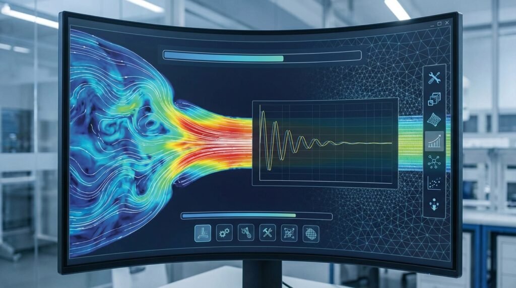
Image: An illustrative graph demonstrating how iterative solutions converge towards a stable point. Source: Wikimedia Commons.

What Exactly Are Convergence Criteria?

Most complex engineering simulations, particularly those involving non-linearity (material, geometric, or contact), solve systems of equations iteratively. This means the solver makes an initial guess, calculates an error or residual, and then refines its guess in subsequent steps until that error falls below a predefined tolerance. Convergence criteria are simply these predefined tolerances or conditions that signal the iterative process can stop because a stable and acceptable solution has been found.

Why Convergence Matters for Your Engineering Models

The impact of convergence goes beyond just getting a numerical answer. It directly affects the:

Accuracy of Results: A non-converged solution might show stresses, deformations, or flow patterns that are numerically unsound and don’t reflect reality.
Reliability and Trustworthiness: Converged results provide confidence in your design decisions, whether for structural integrity assessments (FFS Level 3), aerospace component design, or optimizing oil & gas equipment.
Computational Efficiency: Setting appropriate criteria prevents the solver from running unnecessary iterations, saving time and computational resources. Conversely, too loose criteria can lead to inaccurate answers, negating any time savings.
Model Stability: Ensuring convergence helps to confirm that your model setup (geometry, mesh, boundary conditions, material properties) is robust and physically viable.

Key Types of Convergence Criteria in FEA & CFD

Different physics and solution methods require different criteria. Here are the most common types you’ll encounter:

Residual Convergence

This is perhaps the most fundamental criterion, especially prevalent in CFD and non-linear FEA. Residuals represent the imbalance in the governing equations (e.g., momentum, continuity, energy equations for CFD; force equilibrium for FEA) at each node or element. The solver aims to drive these residuals down to a very small number.

CFD (e.g., Fluent, OpenFOAM): You’ll typically monitor residuals for continuity, momentum (x, y, z), energy, and turbulence equations. Common targets are 1e-3 for basic flow fields and 1e-5 or 1e-6 for energy and species transport, depending on accuracy needs.
FEA (e.g., Abaqus, ANSYS Mechanical): Here, residuals often relate to force or moment equilibrium. The unbalanced force should be a small fraction of the applied load or internal forces.

Displacement/Nodal Variable Convergence

Primarily used in implicit non-linear FEA, this criterion checks the incremental change in nodal displacements (or other nodal variables like temperature or pore pressure) between successive iterations. If the change is very small, it suggests the solution is stabilizing.

Criterion: Ratio of the maximum change in displacement (or other variable) to a characteristic displacement (or variable) value in the model.
Typical Values: Often set to 1e-2 or 1e-3, indicating that successive changes are less than 1% or 0.1% of the total displacement.

Force/Moment Convergence

In FEA, this criterion assesses how well the internal forces balance the external applied loads. It ensures that the system is in equilibrium.

Criterion: Ratio of the out-of-balance force (residual) to the applied force or an average force in the model.
Typical Values: Usually stricter than displacement, 1e-3 to 1e-5 is common.

Energy Convergence

Some solvers monitor the change in the total solution energy between iterations. When this change becomes negligible, the solution is considered converged.

Application: Useful for general non-linear problems, offering a global perspective on convergence.

Solution Variable Convergence (General)

This is a broader term encompassing the monitoring of specific field variables (e.g., velocity, pressure, temperature, stress components) at particular points or globally. When these variables stop changing significantly between iterations, the solution is converging.

Time Step Convergence (for Transient Analyses)

In transient simulations (e.g., explicit dynamics in Abaqus, transient CFD in Fluent, ADAMS multibody dynamics), the solver also needs to determine an appropriate time step. While not a criterion for an iterative solve within a single time step, it’s critical for the stability and accuracy of the overall transient solution. Automatic time stepping algorithms rely on internal convergence checks or stability limits (like CFL number in CFD) to adjust the step size.

Practical Workflow for Achieving Robust Convergence

Achieving convergence isn’t just about setting numbers; it’s an iterative process involving setup, monitoring, and adjustment. Here’s a typical workflow:

1. Pre-Analysis Setup: The Foundation

Geometry Simplification: Remove small features that don’t significantly impact the physics but can cause meshing and convergence headaches.
Mesh Quality: A high-quality mesh is non-negotiable. Ensure good element aspect ratios, skewness, and Jacobian. For contact, refine meshes in contact regions. Tools like Abaqus, ANSYS, and MSC Patran have extensive mesh diagnostic utilities.
Material Properties: Ensure material models are well-defined and physically realistic. Non-linear materials (e.g., plasticity, hyperelasticity) can be very sensitive.
Boundary Conditions & Loads: Apply loads and constraints correctly. Avoid over-constraining or under-constraining the model, which can lead to singularities or rigid body motions.
Initial Conditions: For transient or highly non-linear problems, a good initial guess (e.g., from a simpler linear analysis) can significantly aid convergence.

2. Solver Configuration & Iteration Controls

Select Appropriate Solver: Implicit solvers are generally stable but can struggle with severe non-linearity; explicit solvers are robust for highly dynamic, large-deformation, or contact-rich problems.
Adjust Convergence Tolerances: Start with default or slightly looser tolerances, then tighten them if needed. Don’t go excessively tight initially, as this increases computation time.
Incrementation & Stepping: For non-linear FEA, use small load increments or automatic time stepping (e.g., in Abaqus ‘stabilize’ parameter, ANSYS ‘substeps’).
Stabilization Techniques: Some solvers offer stabilization methods (e.g., artificial damping in Abaqus/Explicit, under-relaxation factors in Fluent/CFX) to help smooth out highly non-linear responses and aid initial convergence. Use with caution as they can mask genuine physical instabilities.
Choose Iterative Solvers Carefully: For large CFD models, the choice of linear solver and its settings (e.g., AMG, GMRES in OpenFOAM) can significantly impact convergence speed and stability.

3. Monitoring & Diagnostics During Solution

Plot Residuals: Always monitor convergence plots provided by your software. Look for a smooth, monotonic decrease in residuals. Fluctuations or plateaus indicate issues.
Monitor Solution Variables: Track key displacements, stresses, temperatures, or velocities at critical points. Do they behave as expected?
Check Warnings/Errors: Solver output often provides crucial clues about element distortion, negative Jacobians, contact penetrations, or numerical instabilities. Don’t ignore them!

Verification & Sanity Checks Beyond Convergence

Even if your solver reports convergence, a critical engineer always performs additional checks to ensure the solution is physically meaningful and accurate.

Mesh Sensitivity Studies

This is a fundamental check. Run your analysis with progressively finer meshes. The results (e.g., peak stress, displacement, lift/drag coefficients) should converge to a stable value. If they don’t, your mesh is too coarse, regardless of solver convergence.

Boundary Condition (BC) & Load Checks

Visualize your BCs and loads. Are they applied correctly? Are there any unexpected reactions or load paths? For example, check reaction forces/moments against applied loads for equilibrium.

Physical Interpretation & Trend Analysis

Does the deformation, stress distribution, or flow field make physical sense? Are stresses concentrated where expected? Is the flow laminar or turbulent in the right regions? Use engineering judgment and hand calculations where possible.

Sensitivity Analysis

Vary key input parameters (material properties, loads, geometry dimensions) within their expected ranges. Observe how results change. An overly sensitive model might indicate a lack of robustness or an issue with your setup.

Comparison & Validation

Wherever possible, compare your simulation results with:

Analytical solutions (for simplified cases)
Experimental data
Benchmark problems
Results from different software packages or modeling approaches

Common Pitfalls and Troubleshooting Convergence Issues

Divergence or false convergence can be frustrating. Here’s how to tackle common problems:

1. Divergence: The Solution Explodes or Fails

Causes: Extreme non-linearity, poor mesh quality, incorrect boundary conditions, large load increments, material model instability, rigid body motion.
Troubleshooting:
- Review BCs: Ensure adequate constraints to prevent rigid body motion. Check for over-constraints.
- Refine Mesh: Especially in regions of high gradients or contact.
- Small Increments: Reduce load/time increments or enable automatic incrementation.
- Stabilization: Add artificial stabilization if the problem is physically quasi-static but numerically unstable (e.g., Abaqus/Standard general contact stabilization).
- Material Properties: Check for negative tangent moduli in non-linear materials.
- Initial Conditions: Provide a better initial guess if possible.

2. False Convergence: The Solution Looks Converged but Isn’t Accurate

Causes: Tolerances set too loosely, oscillations around the solution, solver stopping prematurely.
Troubleshooting:
- Tighten Tolerances: Gradually reduce convergence criteria (e.g., from 1e-3 to 1e-5).
- Monitor Key Variables: Don’t just rely on residual plots; watch how critical output variables change.
- Review Solver Messages: Some solvers might warn about oscillations.

3. Poor Mesh Quality

Impact: Distorted elements lead to inaccurate stiffness matrices (FEA) or poor discretisation (CFD), hindering convergence.
Troubleshooting: Focus on mesh refinement and quality checks (Jacobian, aspect ratio, skewness) in critical areas. Consider using advanced meshing techniques.

4. Contact Non-Linearities

Impact: Complex contact interactions can cause severe non-linearity, chattering, and sudden changes in stiffness.
Troubleshooting:
- Refine Contact Mesh: Ensure fine mesh on contact surfaces.
- Adjust Contact Algorithm: Normal contact stiffness, allowable penetration, stabilization (e.g., in Abaqus General Contact).
- Smooth Surfaces: Avoid sharp corners where contact initiates.
- Small Increments: Load gradually.

5. Material Model Instabilities

Impact: Certain non-linear material models (e.g., rubber-like hyperelasticity, highly plastic metals) can exhibit instabilities if not properly characterized or if strains are too large.
Troubleshooting: Review material curves, ensure they are smooth and physically sound. Use stable integration schemes.

Summary of Common Convergence Criteria & Their Applications

Criterion Type	Typical Application	Common Software	Typical Tolerance Range	Notes
Residual (Force/Moment)	Non-linear Structural FEA (Implicit)	Abaqus, ANSYS Mechanical, MSC Nastran	1e-3 to 1e-5	Checks force equilibrium. Lower values mean stricter convergence.
Residual (Flow, Energy, Species)	CFD Simulations	ANSYS Fluent/CFX, OpenFOAM	1e-3 (Flow), 1e-5/1e-6 (Energy, Species)	Imbalance in governing equations. Often monitored visually.
Displacement Increment	Non-linear Structural FEA (Implicit)	Abaqus, ANSYS Mechanical	1e-2 to 1e-3	Change in nodal displacement between iterations.
Energy Increment	General Non-linear FEA	Abaqus, ANSYS Mechanical	1e-2 to 1e-4	Change in solution energy. Provides a global convergence measure.
Solution Variable (e.g., Velocity, Temp.)	CFD, Heat Transfer FEA	Fluent, OpenFOAM, ANSYS Mechanical	1e-4 to 1e-6	Checks change in specific field variables at points/regions.
Time Step Stability	Transient Explicit Dynamics, Some CFD	Abaqus/Explicit, LS-DYNA, ADAMS	CFL & stability limits (internal)	Not a direct convergence criterion, but critical for transient accuracy/stability.

Best Practices Checklist for Robust Simulation Convergence

Start Simple: Begin with a simplified model or linear analysis, then gradually introduce non-linearities.
Understand Your Physics: Knowing the underlying mechanics helps in interpreting results and troubleshooting.
Quality Meshing: Invest time in creating a good mesh, especially in critical regions and contact zones.
Realistic Boundary Conditions: Ensure loads and constraints accurately represent the physical system.
Monitor Extensively: Don’t just click ‘run’. Actively monitor convergence plots, output variables, and solver messages.
Save Frequently: For long runs, set up frequent saves or restart points.
Document Your Settings: Keep a record of the convergence criteria and solver settings used for each analysis.
Iterate & Refine: Convergence is often an iterative process of adjusting settings, refining the mesh, and re-running.
Leverage HPC: For complex models demanding significant computational power, EngineeringDownloads offers affordable HPC rental services, alongside online courses and project consultancy to help you master these advanced techniques.
Validate: Always perform sanity checks and validation against known results or experiments.

Mastering convergence criteria is a cornerstone of producing reliable engineering simulation results. It’s an art as much as a science, requiring a blend of theoretical understanding, practical experience with software tools, and sound engineering judgment. By diligently applying these principles, you can significantly enhance the quality and trustworthiness of your FEA and CFD analyses for critical applications in structural integrity, biomechanics, and beyond.