Zero Pivot Warning: Your Guide to FEA Stability & Troubleshooting

troubleshooting
Engineering Downlaods
March 13, 2026
22 Minute

Demystifying the Zero Pivot Warning in FEA

As engineers immersed in the world of Finite Element Analysis (FEA), encountering a ‘Zero Pivot Warning’ can be a moment of frustration. It often halts your simulation, preventing you from obtaining crucial results. But what exactly does this warning mean? In essence, a Zero Pivot Warning indicates a fundamental issue with the numerical stability or solvability of your FEA model. It’s the solver’s way of telling you that the system of equations representing your structure is singular, meaning it cannot find a unique solution. This usually points to an under-constrained model or a severe numerical instability.

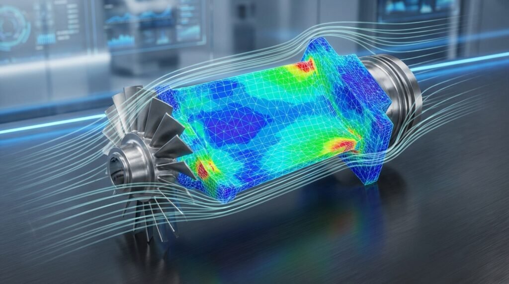
A typical finite element mesh, the foundation of any FEA simulation. Image courtesy of Wikimedia Commons.

Why Zero Pivot Warnings Matter for Engineers

Ignoring or improperly addressing a Zero Pivot Warning can have severe consequences for your engineering projects. These warnings are not minor glitches; they are critical indicators of an unsound model. Here’s why they demand your full attention:

Invalid Results: If the solver manages to proceed despite a warning (sometimes by using stabilization techniques), the results will likely be physically meaningless and unreliable. You cannot trust stress, displacement, or strain predictions from a numerically unstable model.
Failed Analyses: More often, the solver will simply stop, wasting valuable computational time and delaying your project timeline.
Design Flaws: Basing design decisions on flawed simulation results can lead to costly prototypes, structural failures, safety hazards, and reputational damage.
Loss of Productivity: Repeated failures in analysis due to unaddressed zero pivot issues significantly impact your workflow and efficiency.

For structural integrity assessments, failure to find a stable solution can mean the difference between accurately predicting component lifespan (e.g., in FFS Level 3 assessments for oil & gas infrastructure) and making unsafe assumptions. In aerospace and biomechanics, where precision is paramount, these warnings highlight critical model deficiencies that must be resolved before any design validation can occur.

Understanding the Mechanics: What Causes It?

At its core, FEA involves solving a large system of linear algebraic equations, often represented as [K]{u} = {F}, where [K] is the global stiffness matrix, {u} is the vector of unknown nodal displacements, and {F} is the vector of applied nodal forces. A Zero Pivot Warning occurs when the solver encounters a zero or near-zero value on the diagonal of the stiffness matrix during its factorization process (e.g., LU decomposition).

What a Zero in the Stiffness Matrix Diagonal Means

A zero on the diagonal of the stiffness matrix typically corresponds to a degree of freedom (DOF) that has no stiffness associated with it. This implies:

Rigid Body Motion: The most common cause. A part or a significant portion of your model is free to translate or rotate without resistance, meaning it’s not adequately constrained.
Mechanism Formation: Certain combinations of elements and boundary conditions can create local mechanisms, where a small part of the structure can deform without experiencing any resistance.
Incompatible Elements or Material Properties: Sometimes, incorrect element types or material definitions (e.g., specifying zero stiffness properties) can lead to DOFs lacking stiffness.

The solver cannot invert a singular stiffness matrix because its determinant is zero. Geometrically, this means the system has infinite solutions (if consistent) or no solutions (if inconsistent), rather than a unique, stable displacement field.

Common Scenarios & Industries Affected

Zero Pivot Warnings are most prevalent in static structural FEA, but the principles of numerical stability extend to other domains.

Structural Engineering & FEA

Under-constrained Models: Perhaps the most frequent culprit. Missing boundary conditions (BCs) are common, especially in complex assemblies where a component might inadvertently be left floating.
Contact Modeling Issues: Improperly defined contact can lead to initial penetrations or gaps that prevent components from properly constraining each other, causing initial rigid body motion.
Buckling Analysis: In some cases, a zero pivot can indicate that a structure is at a point of instability, approaching buckling.
Material Nonlinearities: Highly nonlinear materials (e.g., hyperelasticity, plasticity) can sometimes lead to numerical difficulties that manifest as solver instabilities.

Beyond Structural FEA

While the term ‘zero pivot’ is specific to stiffness matrix factorization, similar numerical stability issues can arise in other simulations:

CFD (Computational Fluid Dynamics): Solvers like Fluent or OpenFOAM can encounter divergence issues, often due to poor mesh quality, aggressive solver settings, or unstable boundary conditions. While not called ‘zero pivot’, the underlying principle is a lack of numerical stability.
Multibody Dynamics (e.g., ADAMS): Improperly constrained mechanisms can lead to solver errors akin to rigid body motion, where a component has unresisted movement.

Industries like Oil & Gas (pressure vessel analysis, pipeline integrity), Aerospace (aircraft component stress analysis, fatigue life), Automotive (crash simulations, durability), and Biomechanics (implant design, joint mechanics) heavily rely on robust FEA. In all these areas, understanding and resolving zero pivot warnings are crucial for reliable and safe designs.

Diagnosing the Problem: How to Identify Root Causes

Effective troubleshooting begins with a systematic approach. Don’t just guess; follow a diagnostic checklist.

Mesh Quality Issues

A poorly constructed mesh can introduce numerical instabilities. While not a direct cause of *global* rigid body motion, bad elements can cause local stiffness issues.

Distorted Elements: Elements with high aspect ratios, warpage, or Jacobian ratios can lead to poor conditioning of the stiffness matrix.
Zero-Volume Elements: In rare cases, corrupted mesh generation can result in elements with zero volume, effectively removing stiffness from their associated DOFs.

Actionable Tip: Use your pre-processor’s mesh diagnostic tools. Check element quality metrics like Jacobian, aspect ratio, skewness, and internal angles. Ensure there are no collapsed elements or unwanted singularities in the mesh topology.

Boundary Conditions (BCs) and Constraints

This is by far the most common cause. An under-constrained model will always result in a zero pivot.

Insufficient Constraints: The entire model, or a floating component within an assembly, lacks enough fixed DOFs to prevent rigid body motion (translation and rotation). A 3D body needs 6 constraints (3 translational, 3 rotational) to be fully fixed.
Local Under-constraint: A part of the model might be constrained, but a sub-component connected to it is not adequately constrained relative to the main part.
Weak Springs/Connections: If you’re using weak springs or connections to stabilize a model, they might not be stiff enough to prevent a zero pivot, especially if they’re in the wrong direction.

Actionable Tip: Visualize your BCs carefully. Use nodal displacement plots in a preliminary linear static run with minimal load to identify floating components. For assemblies, ensure all parts are connected correctly and that the assembly as a whole is constrained. Consider a ‘fixed boundary’ or ‘fixed base’ condition on a non-load-bearing surface temporarily to check if the model then runs.

Material Properties

Incorrect material definitions can lead to DOFs with zero stiffness.

Zero or Negative Elastic Modulus (E): Entering a non-positive value for Young’s Modulus (E) will result in a stiffness matrix singularity.
Missing Material Definition: Elements might be assigned a non-existent or default material with zero properties.

Actionable Tip: Double-check all material properties. Ensure Young’s Modulus and Poisson’s Ratio are positive and realistic. Verify that all elements in the model have a material assigned.

Element Types

Specific element types, if used improperly, can cause issues.

Incompatible Element Types: Mixing incompatible elements, especially between different regions or in contact, can sometimes lead to numerical issues.
Hourglassing: In continuum elements (solids) with reduced integration, hourglassing can occur if not properly controlled, leading to spurious zero-energy modes that resemble a lack of stiffness.

Actionable Tip: Consult your software’s documentation for recommended element usage. Ensure you’re using appropriate elements for the type of analysis (e.g., shell elements for thin structures, solid elements for bulky ones). If using reduced integration, enable hourglass control.

Solver Settings

Sometimes, the solver’s default settings or advanced options can contribute to or help diagnose the problem.

Numerical Precision: Very small values in the stiffness matrix might be treated as zero if the numerical precision is too coarse.
Stabilization: Some solvers offer artificial stabilization techniques (e.g., weak springs, automatic stabilization). While useful for convergence, they can mask underlying model errors.

Actionable Tip: For initial debugging, consider using a direct solver if available (though computationally expensive) as it can sometimes pinpoint the location of the singularity more directly than iterative solvers. Avoid artificial stabilization until you’ve confirmed your model is structurally sound.

Contact Issues

Poorly defined contact interactions are a frequent source of zero pivot warnings, particularly in assemblies.

Initial Gaps/Penetrations: If contact surfaces start with gaps, they won’t constrain motion until they touch, allowing initial rigid body movement. If they start with excessive penetration, the solver might struggle to resolve the contact.
Insufficient Contact Stiffness: In some formulations, contact stiffness might be too low, failing to prevent relative motion.
Contact Region Definition: Ensure contact pairs or surfaces are correctly defined and cover the intended interaction areas.

Actionable Tip: Use initial step or contact diagnostics to check for initial gaps or penetrations. Adjust contact definitions (e.g., initial adjustments, search distance) to ensure components are either in contact or appropriately separated without allowing free movement.

Practical Workflow for Resolution: Step-by-Step Guidance

Resolving a Zero Pivot Warning requires a methodical approach. Follow these steps:

Pre-analysis Checklist

Model Review: Visually inspect your entire model. Are all parts present? Are there any obvious disconnections?
Units Consistency: Ensure all input units (length, force, stress, material properties) are consistent. Inconsistent units can lead to extremely small or large stiffness values.
Material Properties Check: Verify all materials have positive and realistic Young’s Modulus and Poisson’s Ratio.
Boundary Conditions Review: Confirm sufficient constraints. For a single component, ensure 6 DOFs are constrained. For assemblies, ensure the entire assembly is fixed, and all components are adequately connected to each other.
Connections & Interactions: Check all connections (bolts, welds, contact surfaces) to ensure they are properly defined and truly connect parts.
Mesh Quality Report: Run mesh quality checks and address any severe distortions or failed elements.

Iterative Debugging Process

If the pre-analysis checks don’t resolve the issue, proceed with these iterative steps:

Start Simple: If you’re working with a complex assembly, try running a simulation on an isolated component with simplified boundary conditions. If it runs, the issue is likely with the assembly or its connections/BCs.
Gradual Constraint Application: For a complex model, try adding very stiff springs (or even fixed constraints temporarily) at key locations to prevent rigid body motion. If the model then runs, gradually relax these constraints or replace them with more realistic ones until the problem reappears, helping you pinpoint the problematic region.
Rigid Body Mode Extraction: Many FEA solvers (Abaqus, ANSYS Mechanical, Nastran) have a feature to extract rigid body modes (eigenvalues near zero). This can graphically show you which parts of your model are unconstrained. This is an invaluable tool for diagnosis.
Submodeling/Substructuring: For very large models, isolate problematic regions into smaller submodels to debug more efficiently.
Small Load Application: Apply a very small, non-physical force in the suspected direction of free movement. If it results in extremely large displacements, it confirms unconstrained rigid body motion.
Contact Diagnostics: If contact is involved, run a simple contact analysis or use contact visualization tools to ensure surfaces are engaging as intended.
Solver Output Log: Thoroughly read the solver’s output file or log. It often contains detailed messages about the location (node, element, DOF) where the zero pivot occurred. This is your most direct clue.

Tool-Specific Considerations

While the underlying principles are universal, different FEA packages present and help diagnose zero pivot warnings in their own ways.

Abaqus

Warning Message: Abaqus often reports ‘numerical singularities’ or ‘zero pivot’ warnings, sometimes pointing to specific nodes or DOFs.
Debugging Tools: The ‘Job Diagnostics’ and ‘.dat’ file are crucial. Abaqus can also output ‘eigenvalues of the stiffness matrix’ at the beginning of an analysis, with values near zero indicating rigid body modes.
Stabilization: Abaqus offers ‘Automatic Stabilization’ (*CONTROLS, STABILIZE) which can help converge but should be used cautiously as it adds artificial stiffness.

ANSYS Mechanical

Warning Message: ANSYS often reports ‘singular matrix’, ‘pivot warning’, or ‘small pivot’ messages, sometimes indicating the element or node involved.
Debugging Tools: The ‘Output Window’ in Mechanical or the ‘.out’ file provides detailed solver messages. Use the ‘Unconstrained Body Motion’ diagnostic tool (often under ‘Solution Information’ or ‘Solver Output’ options) which attempts to find and animate rigid body modes.
Springs: ANSYS allows adding weak springs to specific nodes or components to temporarily stabilize the model.

MSC Patran/Nastran

Warning Message: Nastran typically provides ‘FATAL’ errors like ‘U.M.’ (unsupported mass) or ‘singular stiffness matrix’ in the ‘.f06’ file.
Debugging Tools: The ‘.f06’ output file is the primary source of information. Nastran has a ‘SOL 103 (Modal) analysis’ which, if run with no boundary conditions, will show 6 rigid body modes with near-zero frequencies. If more than 6 modes are near zero, it indicates a mechanism or an unconstrained part.
AutoSPC: Nastran’s PARAM, AUTOSPC, YES can automatically constrain unsupported DOFs, but again, this should be used for debugging, not as a permanent fix.

Verification & Sanity Checks

After resolving the zero pivot warning, it’s crucial to verify the integrity and accuracy of your simulation.

Convergence Criteria

A successful run doesn’t automatically mean accurate results. For nonlinear analyses, check the convergence plots. Ensure the solution converged within the specified tolerances for force and displacement.

Sensitivity Analysis

Perform a sensitivity analysis on your boundary conditions or material properties. Small changes should lead to reasonable, predictable changes in results. If results drastically change with minor input variations, it might indicate remaining numerical instability or a sensitive design.

Result Interpretation & Validation

Displacement Plots: Visually inspect displacement contours. Are they physically realistic? Are there any extreme, localized displacements that seem incorrect?
Stress Plots: Check stress concentrations. Do they align with engineering intuition? Are stress values reasonable for the applied loads and material?
Reaction Forces: Sum up reaction forces at constraints and compare them against applied loads to ensure equilibrium.
Hand Calculations/Benchmarking: Whenever possible, perform simplified hand calculations or compare your results against known benchmarks or experimental data.

These checks are fundamental for building confidence in your simulation output, especially vital for critical applications like FFS Level 3 assessments where safety margins are calculated based on these results.

Prevention Strategies: Best Practices for Robust Models

Preventing zero pivot warnings is always better than troubleshooting them.

FEA Modeling Best Practices

Start with Simplicity: Begin with a simplified model, get it to run, then gradually add complexity (nonlinearities, contacts, intricate geometry).
Clear Constraint Strategy: Before modeling, have a clear plan for how your structure will be constrained. For assemblies, define how each component interacts and is constrained relative to others.
Use Symmetric Constraints: When appropriate, leverage symmetry boundary conditions to reduce model size and simplify constraints.
Review Connections Rigorously: For assemblies, ensure all connections (contact, fastened connections, welds) are properly defined and fully constrain relative motion where intended.
Pilot Loads/Test Runs: Perform small, simple pilot runs with basic loads to check for fundamental model stability before applying complex loading scenarios.

Modeling Tips for Complex Scenarios

When dealing with advanced setups:

Nonlinear Contact: For contact, consider using a “smooth” initial contact rather than allowing large penetrations. Use “tied contact” or “bonded contact” for areas meant to be permanently joined.
Implicit vs. Explicit: For highly nonlinear or dynamic problems with significant contact, consider if an explicit solver might be more appropriate, as they handle contact and large deformations differently and avoid forming a global stiffness matrix.
Element Order: Generally, higher-order elements (e.g., quadratic) offer better accuracy but can be more sensitive to mesh distortion. Test linear vs. quadratic elements for stability.

Advanced Troubleshooting Techniques

Sometimes, simple fixes aren’t enough. Here are a few advanced techniques:

Matrix Conditioning

A badly conditioned stiffness matrix can lead to numerical instability, even if strictly non-singular. This often arises from extreme differences in material stiffness or element sizes within the same model.

Identify Stiff/Soft Regions: Look for areas with vastly different stiffnesses. This can be problematic for iterative solvers.
Scaling: Ensure your model’s dimensions and material properties don’t lead to excessively large or small numbers in the matrix. Consistent units are key.

Stabilization Methods

While artificial stabilization can mask problems, in some truly difficult nonlinear contact problems (e.g., sheet metal forming), it might be a necessary tool, provided its impact on results is understood and minimal.

Viscous Damping: Introducing a small amount of viscous damping can help numerical convergence in dynamic problems or quasi-static problems with severe contact.
Weak Springs: Small, artificial springs can be added to initially stabilize a model, especially during initial contact engagement. These should be weak enough not to significantly alter the physics.

Leveraging Python & MATLAB for Diagnosis & Automation

For advanced users, scripting languages like Python and MATLAB can be powerful allies in diagnosing and preventing zero pivot warnings.

Pre-processing Checks

Automated BC Verification: Write Python scripts (e.g., using Abaqus scripting interface or ANSYS PyMAPDL) to automatically check if all desired DOFs are constrained or if any nodes are isolated.
Material Property Scan: Develop scripts to scan input files for suspicious material properties (e.g., E = 0, negative Poisson’s ratio).
Mesh Quality Reporting: Integrate mesh quality checks into automated pre-processing routines to flag poor elements before submission.

Post-processing Diagnostics

Rigid Body Mode Visualization: If your solver provides modal analysis output, Python or MATLAB can be used to process and visualize near-zero frequency modes more effectively, highlighting unconstrained regions.
Displacement Extremes: Scripts can identify nodes with excessively large displacements that might indicate an unconstrained region, even if the solver didn’t fully stop.

For complex cases or to develop custom Python/MATLAB scripts for these checks, explore the expert tutoring and consultancy services available at EngineeringDownloads.com. Our specialists can help you implement robust automation strategies for your CAD-CAE workflows.

Key Takeaways & Best Practices Checklist

To summarize, tackling Zero Pivot Warnings boils down to vigilance and systematic problem-solving:

Problem Type	Common Causes	Actionable Solutions	Verification Step
Under-constraint	Missing or insufficient BCs, floating components, weak connections.	Add appropriate fixed BCs, use rigid body mode extraction, simplify model for debugging.	Run linear static analysis, check reaction forces and displacements.
Material Issues	Zero/negative Young’s Modulus, missing material assignments.	Verify all material properties, ensure assignment to all elements.	Review input file/pre-processor material definitions.
Mesh Quality	Distorted elements, zero-volume elements, poor aspect ratios.	Improve mesh quality (remesh problematic areas), enable hourglass control.	Run mesh quality checks, visually inspect problem areas.
Contact Problems	Initial gaps/penetrations, incorrect contact definitions, insufficient contact stiffness.	Adjust initial contact conditions, refine contact pairs, verify contact regions.	Run contact diagnostics, visualize initial contact status.
Solver Instability	Aggressive solver settings, very nonlinear problems, poor matrix conditioning.	Use direct solver for diagnosis, consider explicit solvers for highly nonlinear problems, adjust solver tolerances.	Check solver log for convergence, perform sensitivity analysis.

Remember, a Zero Pivot Warning is a critical signal that your model needs attention. Address it systematically, understand its root cause, and verify your solutions to ensure the integrity and accuracy of your engineering simulations.