Thermal stress analysis is the process of evaluating mechanical stress caused by temperature changes in materials and structures. When materials heat up, they tend to expand; when they cool down, they contract. If this expansion or contraction is unconstrained, the material simply changes size without any stress. But if parts of a structure are restrained from moving (for example, a steel beam fixed at both ends), thermal expansion or contraction is hindered – and internal stresses develop. These thermal stresses can be large enough to cause serious issues like cracks, warping, or even total failure of components if not accounted for. In simple terms, when a structure wants to expand or shrink due to a temperature change but cannot freely do so, stress builds up – that’s thermal stress.

In this friendly guide, we’ll start from the basics of thermal stress in engineering and gradually move to advanced finite element modeling techniques. We will explain why thermal stress analysis is important, how to calculate thermal stresses with simple formulas, and the different types of thermal stress analyses (linear vs nonlinear, uncoupled vs coupled). Importantly, we’ll provide guidance on how to perform thermal stress analysis using popular FEA tools – focusing on Abaqus and ANSYS, with mentions of others like COMSOL and CalculiX. By the end, you’ll understand not only what thermal stress analysis is, but also how to carry it out in practice, and why it’s crucial for safe and reliable designs. Let’s dive in!

1. What is Thermal Stress Analysis in Engineering?

Thermal stress analysis is all about figuring out how much stress a material or structure experiences due to temperature changes. In engineering, most materials expand when heated and shrink when cooled. This behavior is quantified by a material property called the Coefficient of Thermal Expansion (CTE), often denoted as α, which tells us how much a material expands per degree of temperature increase. If a component is free to expand (nothing is holding it back), then a temperature rise just makes it a bit larger, and no stress is induced. However, if that component is constrained (attached to other parts or fixed in place), it cannot expand freely – and that’s when thermal stresses occur.

Why does heating or cooling cause stress? Consider a simple example: a glass jar with a metal lid. When you run hot water over the metal lid, it expands slightly; the glass jar, being cooler, doesn’t expand as much. The difference in expansion can make the lid easier to twist off. Now imagine the lid were somehow prevented from expanding – the heating would generate stress in the metal. On a larger scale, imagine a long steel beam tightly bolted at both ends. If the temperature increases significantly and the beam wants to elongate, the rigid attachments will resist the expansion, causing compressive stress in the beam (and tensile stress in whatever is holding it). On cooling, the opposite happens – the beam wants to contract, and if held fixed, it will develop tensile stress. This simple concept – thermal expansion + constraint = stress – is the core of thermal stress analysis.

To visualize the effect, picture a railway track on a scorching day. Rails are often installed with small gaps or expansion joints. Without these, the rails can heat up and expand, eventually bowing or buckling under compressive thermal stress. In fact, a 100-foot (30 m) steel pipe heated by about 100 °C (from, say, room temperature to ~200 °F) can exert over 120,000 pounds of force if it’s constrained from expanding! That immense force can easily warp or damage structures. Thermal stress analysis helps engineers predict such outcomes and design measures (like expansion joints, allowable gaps, or flexible supports) to prevent damage.

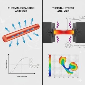
1.1 Thermal Expansion vs Thermal Stress – What’s the Difference?

It’s important to distinguish thermal expansion from thermal stress:

• Thermal Expansion Analysis (Heat Transfer Analysis) – focuses on how temperature changes cause dimensional changes. Essentially, it answers “How does temperature spread through a material, and how much expansion or contraction results?” This is typically a pure heat transfer analysis: you compute the temperature distribution (for example, using conduction, convection, and radiation principles) and the free expansion that would occur.
• Thermal Stress Analysis – focuses on the stresses and deformations that result because of those temperature changes (when expansion is restrained). It answers “Given the temperature change in a material, what stresses (and possibly strains or displacements) occur due to thermal expansion being constrained?”. In practice, thermal stress analysis often uses the results of a heat transfer analysis as input.

In summary, a typical engineering approach is: first do a heat transfer analysis to find the temperature field, then do a structural analysis to find stresses caused by that temperature field. Many FEA tools (like Abaqus, ANSYS, COMSOL) allow you to do this sequentially, or even simultaneously in a coupled simulation. We will explore these methods later in the guide.

2. Why Do We Need Thermal Stress Analysis?

Thermal stresses can be invisible killers in engineering designs. We need thermal stress analysis to catch problems that purely mechanical or static analysis might miss. When temperature changes create internal forces, a structure can fail even if no external load is applied! Here are a few reasons why thermal stress analysis is crucial:

• Preventing Cracks and Structural Failures: If engineers ignore thermal stress, the results can be disastrous. Brittle materials like glass or ceramics can crack from thermal shock – for instance, pouring cold water onto hot glass can make it shatter due to rapid contraction at the surface. Metals can undergo thermal fatigue if repeatedly heated and cooled, forming cracks over time. A classic example is a welded component: as it cools after welding, uneven contraction can leave residual stresses and cracks if not properly managed.
• Avoiding Warping and Deformation: Components may warp or buckle when thermal expansion is constrained. Imagine a long bridge in a region with hot summers and cold winters. If expansion joints were not included, the bridge girders could bend or crack as they expand in summer and contract in winter. Pipelines also use expansion loops or joints to accommodate thermal growth; otherwise, they’d rupture or pull on their anchors. Thermal stress analysis helps predict how much a structure might deform under thermal loads, so we can design allowances for that movement.
• Maintaining Performance and Reliability: Thermal stresses can reduce the service life of components. In electronics, for example, silicon chips and circuit boards experience heating during operation. If a chip and the board have different expansion rates, the solder joints between them see cyclic thermal stresses, potentially causing fatigue and electrical failure over time. In high-temperature machinery like jet turbines or automotive engines, parts undergo constant thermal cycling. Ignoring these stresses could mean unexpected failures, costly maintenance, or unsafe operation. By analyzing thermal stresses, engineers ensure components remain within safe stress limits throughout operating temperature ranges, thereby improving reliability.

In short, thermal stress analysis is needed to catch problems that pure thermal or pure mechanical analysis would overlook. It is a safeguard against failure: by understanding where and how temperature changes induce stress, we can design safer and more durable systems. Skipping it might save time initially, but can lead to cracked glass, warped beams, leaking seals, or other failures down the line.

2.1 Real-World Examples of Thermal Stress Problems

It helps to look at some real-world scenarios where thermal stress analysis plays a key role:

• Bridges and Buildings: Ever notice the gaps in bridge segments or railway tracks? These expansion joints are there to accommodate thermal expansion. Without them, a bridge could literally push itself apart or buckle on a hot day. Structural engineers perform thermal stress analysis to determine the size and spacing of expansion joints so that bridges and long buildings can expand/contract safely with temperature.
• Power Plants and Engines: Turbine blades in jet engines or power plant turbines face extreme heat. During operation they heat up and expand; when shut down, they cool and contract. This thermal cycling induces stress that can lead to creep (permanent deformation at high temperature) or fatigue cracking over time. Thermal stress analysis is used to predict blade deformation and stress over a range of temperatures so engineers can select materials and cooling strategies to avoid failure.
• Electronics: A computer’s circuit board has many materials (silicon chips, copper, solder, epoxy board) each with different CTEs. When the device heats up, these materials expand differently. If the design doesn’t account for that, solder joints or components can crack (a common failure mode in electronics called thermal stress fracture). Engineers use thermal stress analysis (often coupled with thermal cycling tests) to ensure reliability of electronic packages – for example, avoiding designs that put too much stress on solder balls in a BGA (ball grid array) due to expansion mismatch.
• Manufacturing Processes: Processes like welding, casting, or heat treating involve rapid heating and cooling. Welding is a prime example: the intense heat causes localized expansion; as the weld cools, it contracts and can pull on the surrounding metal, creating residual stresses and sometimes cracks. A sequential thermal-stress analysis of a weld can predict distortion and residual stress pattern, which helps in planning welding sequence or post-weld heat treatment. Another example is glass manufacturing – as glass cools, if it cools unevenly it can crack from thermal stress. Glassmakers carefully control cooling rates (annealing) based on thermal stress calculations.

The bottom line: thermal stresses are everywhere, from the small scale (microchips) to the large scale (bridges). By performing thermal stress analysis, engineers can foresee where problems might occur and mitigate them – for instance, by choosing materials with compatible expansion rates, adding expansion joints, using insulation, or controlling temperature changes more gradually.

3. How Do We Calculate Thermal Stress? (The Basics)

Thermal stress calculations typically start with a simple idea: thermal strain (the amount a material would expand or contract due to a temperature change) and how that strain is constrained by the material or structure. For small uniform temperature changes and linear materials, one fundamental equation is:

• Thermal Strain: ε_thermal = α · ΔT

Here α is the coefficient of thermal expansion (CTE) and ΔT is the change in temperature. This tells us the fraction of length change per degree. For example, if α = 12×10^-6 (for steel) and ΔT = 50°C, the free thermal strain is 12×10^-6 * 50 = 6×10^-4 (i.e., a 0.06% increase in length if free to expand).

Now, if that strain is fully restrained (the material is not allowed to expand at all), it will turn into a stress according to Hooke’s law (for linear elastic behavior):

• Thermal Stress: σ_thermal = E · α · ΔT

Here E is Young’s modulus (elastic stiffness). This formula essentially comes from σ = E · ε, using ε = αΔT. It gives the stress that develops in a completely locked-up part for a uniform temperature rise ΔT. For instance, using the steel example above (E ~ 210 GPa, α = 12e-6, ΔT = 50°C): σ = 210e9 * 12e-6 * 50 ≈ 126 MPa of stress would be generated if the steel is fully constrained from expanding. If the temperature drops by 50°C (ΔT = –50), the stress would be tensile 126 MPa (trying to pull the material apart).

Important: The above calculation is a simplification – it assumes the whole part is at a uniform ΔT and fully constrained. In reality, temperature might vary across the part (temperature gradients) and only certain directions might be constrained. The actual stress distribution can then be much more complex.

For non-uniform temperature changes, we often integrate the thermal strain over the structure or solve it with FEA. For example, if one end of a rod is hotter than the other, it will expand more on that end, causing bending or differential stress along the rod. These cases require solving differential equations of heat conduction plus elasticity – which is exactly what FEA software does.

Also, material behavior matters. The above formula assumes a linear elastic material (and no phase changes, etc). If the temperature change is large enough to cause plastic deformation or if the material’s properties change with temperature (common at high temps), then a nonlinear analysis is needed (more on that in the next section).

In summary, to hand-calc thermal stress you start from thermal expansion strain (αΔT) and then figure out how the structure’s constraints convert that strain into stress. Simple cases like a uniformly heated, fully fixed rod can be done with one formula. More complex cases (like temperature gradients or partial constraints) usually require solving equilibrium equations – which is where numerical methods (FEA) come in handy.

Modern engineering practice relies on simulation tools to calculate thermal stress for complex geometry and conditions, because they can handle varying temperatures across the part and material nonlinearities. Still, that basic formula is useful for sanity checks. For example, if an FEA result shows 500 MPa thermal stress in a steel part for a 50°C uniform heating, you’d suspect something’s off, because the back-of-envelope calc (EαΔT) gave ~126 MPa. Hand calculations and simple formulas thus provide a reality check for simulation results.

4. Types of Thermal Stress Analysis (Linear vs Nonlinear, Uncoupled vs Coupled)

Not all thermal stress problems are analyzed the same way. We can classify thermal stress analyses based on two main considerations: material/behavior linearity and thermal-structural coupling. Understanding these types will help you choose the right approach for a given problem.

4.1 Linear vs Nonlinear Thermal Stress Analysis

• Linear Thermal Stress Analysis: This assumes everything remains in the linear range – both in terms of material behavior and small deformations. Material properties (like E, α) are treated as constant (usually taken at a reference temperature), and the resulting strains are small enough that geometry doesn’t significantly change. Linear analysis is typically acceptable for moderate temperature changes where the material stays elastic and the structure doesn’t deform drastically. For example, analyzing thermal stress in an aluminum antenna dish under a 30°C ambient change could be linear – aluminum’s expansion is linear with temperature and stresses might remain below yield. Linear analysis is simpler and faster because it often can be solved in one go (and superposition applies). However, it might overpredict stress if the material would actually yield (plastic deformation relieves some stress).

• Nonlinear Thermal Stress Analysis: This comes into play when material properties depend on temperature, when temperatures cause yielding or other nonlinear material behavior, or when large deformations or contact are involved. Nonlinear analysis means the FEA will iterate because, for example, E might decrease as temperature rises (making the structure more compliant), or the material might start yielding at hot spots (capping the stress). A common scenario is rocket engine or turbine components: at high temperatures, metals soften (E drops) and can creep; also thermal strains can be huge, causing plastic deformation. Another scenario is thermal stress with contact – imagine two parts bolted together with a gap, and thermal expansion causes them to press and generate contact pressure; that’s inherently nonlinear (contact conditions changing). Radiation boundary conditions also make the heat transfer nonlinear (since radiative heat transfer ∝ T^4). Nonlinear thermal stress analysis is more realistic for extreme conditions but requires more material data (like stress-strain curves at different temperatures) and more computation time.

In short, linear analysis is fine for small to moderate temperature differentials and elastic response, whereas nonlinear analysis is needed for high-temperature problems, or whenever you expect material or geometric nonlinearity. Always ask: “Will my material or structure behave nonlinearly due to this temperature change?” If yes (or if unsure), a nonlinear analysis is safer. Modern tools like Abaqus and ANSYS allow you to include temperature-dependent properties easily, and will automatically iterate if yielding or large deflection occurs.

4.2 Uncoupled vs Coupled Thermal-Structural Analysis

This is about how we handle the interaction between the temperature field and the stress/deformation field. There are three common approaches:

• Uncoupled Analysis: In an uncoupled approach, you assume that the temperature field is determined independently, without any influence from the structural response. In practice, this means you first solve a pure heat transfer problem (maybe a steady-state or transient thermal analysis) to get the temperature distribution. Then you apply those temperatures as loads in a structural analysis to find the stresses. The key assumption is that the structural deformations or stresses don’t feed back to alter the temperature field. This is often valid when mechanical effects (like deformation) don’t significantly affect heat flow – which is true for many problems. For example, heating a metal bar: unless it deforms so much that it changes convection or contact, the temperature solution is just from the thermal inputs. Uncoupled thermal stress analysis is efficient and simpler (two separate analyses). It’s the most common approach when thermal expansion causes stress but thermal conditions are one-way (i.e., temperature affects stress, but stress doesn’t affect temperature).
• Sequentially Coupled Analysis: This is actually a form of uncoupled analysis done in sequence, but it’s worth mentioning because many FEA workflows use the term “sequential coupling.” It means the same as above – you do thermal first, structural second – but often implies a step-by-step transfer for transient problems. For instance, if you have a time-dependent heating and you want to capture stresses over time, you might run a transient thermal simulation (getting temperature vs time), then at certain time points feed those into a stress simulation. Some software will automate this chaining. In Abaqus, a “sequentially coupled thermal-stress analysis” involves running a heat transfer analysis job, then using its results as a predefined field of temperature in a subsequent stress analysis job. In ANSYS Workbench, you might link a Thermal Transient analysis to a Static Structural analysis via “Load Transfer”. The important thing is, sequential coupling is still a one-way street: the thermal solution is computed first on its own and is then passed over to the structural model. This works great if, for example, you are heating a part and want to know stress at each moment, but the heating itself isn’t altered by the stress.
• Fully Coupled Analysis: In a fully coupled thermal-stress analysis (also called thermo-mechanical coupling), the thermal and mechanical equations are solved together at the same time. In other words, at each time step (or each iteration), the solver considers how the temperature field affects the deformation and how the deformation (or stress) feeds back to affect the temperature field. This two-way coupling is necessary when the interactions are significant. When would stress/deformation affect temperature? One common case is deformation-induced heating: for example, during plastic deformation at high strain rates (like in metal forming or crash simulations), the material heats up due to energy dissipated as heat (this is called adiabatic heating in plastic work). Another case: contact thermal resistance – if two surfaces press together, they conduct heat better; if they separate, heat flow drops. So the contact pressure (a structural result) influences temperature distribution. Frictional heating is another coupled effect (friction generates heat which raises temperature, possibly altering material properties and stresses). For such problems, a fully coupled approach is needed because the thermal solution at a given moment depends on the current deformation state and vice versa. In FEA, fully coupled analysis typically uses special coupled elements (e.g., in Abaqus you use elements that have both temperature and displacement degrees of freedom). The solver will simultaneously solve the matrix equations for both fields. This is more computationally intensive than sequential, but for certain problems (like a rapid metal forging or a brake disk heating and deforming under friction), it’s the only accurate way.

To summarize coupling: if your problem’s physics is such that thermal loads cause stress, but stresses don’t affect thermal loads, then an uncoupled (or sequential) analysis is sufficient (and easier). If instead thermal and mechanical effects influence each other, you need a fully coupled analysis. A handy rule cited in Abaqus documentation is: fully coupled thermal-stress analysis is needed when the stress distribution depends on temperature and the temperature distribution also depends on the stress/deformation solution. If only the former is true (temperature affects stress, but not vice versa), sequential analysis is fine.

It’s worth noting that many practical engineering problems are indeed one-way: for example, thermal expansion in a bridge (the bridge deforming doesn’t change the weather!). But some are two-way: like a press fit (thermal expansion puts pressure which changes thermal contact conductance, albeit a subtle effect). Experienced analysts will judge which approach is needed. Modern multiphysics-capable software (like COMSOL) often encourages fully coupled analysis by default, whereas general FEA tools like Abaqus/ANSYS let you choose.

• Adiabatic and Other Special Cases: There is a special scenario called adiabatic thermal stress analysis, often relevant in fast events (explosions, impacts). “Adiabatic” means no heat transfer out of the material during the event. For instance, in a high-speed impact, plastic deformation heats the material, but the process is so fast that heat doesn’t have time to conduct away – so all that energy stays as a temperature rise in the material, affecting its yield strength. Abaqus has an adiabatic option, which essentially couples plastic work to a temperature increase without solving heat diffusion. It’s like a one-way coupling in the mechanical solver itself (temperatures evolve due to deformation, but you assume no time for conduction). This is a subset of fully coupled analysis, used for problems like ballistic impacts or metal forming where deformation is quick. We mention it because you might come across the term “adiabatic analysis” – it’s a way to include deformation heating without the overhead of solving full heat transfer equations, under the assumption that the process is too fast for significant heat exchange.

Now that we have the conceptual groundwork, let’s see how to actually perform thermal stress analysis using FEA software, specifically Abaqus and ANSYS – two of the most popular tools in this area. We’ll cover the typical workflows for uncoupled vs coupled analyses in these programs, and highlight any special considerations for each.

5. How to Perform Thermal Stress Analysis in Abaqus

Abaqus is well-known for its capabilities in both structural and thermal analysis, and it allows all the approaches discussed (uncoupled, sequential, fully coupled, etc.). Here’s a step-by-step outline of how you would tackle a thermal stress problem in Abaqus:

5.1 Uncoupled Thermal Stress Analysis in Abaqus (Thermal then Structural):
In Abaqus, an uncoupled approach means doing a heat transfer analysis separately from the stress analysis. You would:

1. Set up a Heat Transfer Model: Create your geometry and mesh as needed. Choose a Heat Transfer procedure (either Transient or Steady-State depending on the scenario). Define thermal material properties (like conductivity, specific heat if transient, density, etc.). Apply thermal boundary conditions: e.g., temperatures on certain regions, convection film conditions, heat flux, radiation surfaces, etc. Run this analysis using Abaqus/Standard (implicit solver) because Abaqus/Standard supports heat transfer steps. The result will be a temperature field (as a function of time, if transient).
2. Set up a Structural Stress Model: Now you create a static stress analysis model of the same part. (Often you can use the same mesh if compatible, or Abaqus allows importing the mesh from the thermal model.) Choose a Static or General procedure for stress analysis (or Dynamics if needed). Here, the key step is to import the temperature results from the heat transfer analysis. In Abaqus, you do this by defining a Predefined Field of type Temperature and selecting From File, pointing it to the output database (.odb) of the thermal analysis. You can pick the step and increment (or time) of the thermal simulation that you want to import. These imported temperatures act as applied thermal loads in the stress analysis. Also, make sure your structural material definition includes the coefficient of thermal expansion α (and ideally temperature-dependent α if significant) so that Abaqus knows how much thermal strain to generate. Finally, apply any mechanical boundary conditions (supports, etc.) and loads (if any beyond thermal). Then run this stress analysis (which could be Abaqus/Standard or Abaqus/Explicit depending on needs, though Standard is typical for static analysis).
3. Results: The output will show stress (and deformation) caused by the temperature field. Since we imported the temperature from the first step, the structural analysis will calculate thermal strain = α ΔT and resulting stresses given the constraints. In an uncoupled run like this, the temperatures do not change during the stress analysis – they’re fixed inputs (hence predefined field in Abaqus terms, meaning they aren’t affected by the solution). This is exactly what we expect for a one-way analysis.

This sequential workflow is very common. For example, Abaqus documentation and tutorials often demonstrate it with a two-step process: first a transient heat transfer on a part (say a pipe heating up), then a static stress step that reads those temperatures. In the Technia blog example of an expansion joint, they did a steady-state thermal analysis of a pipe, then applied the resulting temperature as a load in a static analysis to see stresses and the need for an expansion joint. Abaqus makes this easy by using the .odb result mapping – it will map node temperatures from the thermal mesh to the structural mesh automatically (assuming same mesh or it interpolates if needed).

Tips: Ensure the time output you need is saved in the thermal run (if transient). Also, if using Abaqus/Explicit for the stress analysis (say for a very fast event), note that Explicit can’t directly read an .odb from Standard, but you can have Standard write a results file (.fil) or use the restart mechanism. However, typically both steps are done in Standard for convenience unless there’s a special reason to involve Explicit (like extremely short-duration events or highly nonlinear dynamics).

5.2 Fully Coupled Thermal-Stress Analysis in Abaqus:
For a fully coupled analysis, Abaqus provides a procedure called Coupled Temperature-Displacement. Instead of two separate analysis jobs, you set up one analysis that has both thermal and mechanical degrees of freedom active simultaneously. Steps:

1. Coupled Analysis Step: In Abaqus CAE, you’d choose a coupled temperature-displacement step (available in both Standard and Explicit). This step will solve the heat transfer and stress equations together. You need to use element types that have both temperature and displacement d.o.f (for example, in 3D, Abaqus has C3D8T or C3D8RT elements – the “T” indicates thermal coupling). Select those for your mesh.
2. Material Definitions: Provide both sets of properties – thermal (conductivity, specific heat, etc.) and mechanical (elastic modulus, thermal expansion coefficient, yield etc). Also, if plastic deformation is expected with adiabatic heating, you can specify what fraction of plastic work converts to heat (Abaqus uses a default inelastic heat fraction, often 0.9, meaning 90% of plastic work becomes heat).
3. Boundary & Initial Conditions: Now you apply both kinds of conditions. Thermal BCs like before (temperatures, convective film, heat flux) and mechanical BCs (supports, forces, pressures, etc.) can all be applied in the same step or separate steps, but often they act together. For example, a coupled simulation of a braking event might apply a rotational velocity (mechanical) and a contact with friction (which generates heat, thermal) all in one coupled step – the frictional work raises temperature, which causes expansion, which changes contact pressure, etc., all captured together. If using Standard, you can do transient or steady-state coupled analysis. If using Explicit, note that it inherently does transient (no steady state in explicit).
4. Run and Monitor: Coupled problems can be tougher to converge in implicit (Standard) because of the interactions, but Abaqus is designed to handle many. The output will give you both temperature results and stress results over time. You can watch how, say, a part heats and simultaneously deforms.

As an example scenario for fully coupled analysis: imagine hot forging a metal part. The workpiece is hot and being deformed by a press; the deformation generates additional heat and the contact between the die and workpiece conducts heat. A coupled analysis would capture the increase in workpiece temperature from deformation (adiabatic heating) and how the cooling into the dies happens, all while computing the stress and shape change in the metal. Abaqus/Explicit is often used for such problems due to severe deformations and contact, using coupled temperature-displacement elements so that it calculates the temperature rise from plastic work. Abaqus/Standard could also do it (especially for slower processes or smaller strains).

Note: In fully coupled analyses, the mechanical strains can feed back to thermal via two main routes – changing the contact or boundary conditions (like gap conductance), or via heat generation (like plastic heat). However, if your scenario doesn’t actually have those two-way effects, a fully coupled simulation may be overkill. For instance, you can run a coupled analysis of a simple heating just to get stress, but it will give the same result as a sequential approach (just slower) if there’s truly no feedback. Use coupled when needed.

Abaqus is pretty advanced here – it even lets you mix approaches. For instance, you could do a sequential analysis but still consider temperature-dependent material properties (which is a kind of one-sided coupling where the thermal solution is one-way but the stress solution uses updated properties per temperature). That’s common: you run heat transfer, then in the stress step, Abaqus can interpolate, say, the Young’s modulus at each integration point based on that point’s temperature (if you provided a table of E vs T). This accounts for material softening from heat without doing a fully coupled solve.

5.3 A Quick Example (Sequential Coupling in Abaqus):
To cement the idea, let’s outline a quick example many Abaqus users encounter – welding two metal plates. Suppose we weld along the seam of two steel sheets. The welding is a highly localized heat input that raises temperature near the seam above steel’s melting point, then it cools down. We want to know the resulting distortion and residual stress.

• We perform a transient thermal analysis: model the moving weld heat source (or an equivalent thermal load) and simulate the temperature rise and subsequent cool-down. This gives a time-history of temperature in the plates. We likely use Abaqus/Standard for this step (thermal transient).
• Next, we perform a stress analysis: we take the temperature history and apply it to the structural model. In Abaqus, one way is to use the Sequentially Coupled Thermal-Stress analysis technique where you tell the stress step to read temperatures from the thermal step’s results at each time increment[28]. Abaqus can do that in one go if set up properly (read Dependent Field output) or by running separate analysis and importing fields stepwise. The structural analysis (perhaps using Abaqus/Standard static steps or Abaqus/Explicit if the process is highly dynamic) will output the deformation of the plates after cooling and the residual stresses locked in.
• This is sequential coupling because we assumed the welding heat itself is not affected by how the plates deform during welding (a fair assumption if fixtured, etc.). If we wanted to go a step further, we could include the effect of deformation on the welding process (for example, if the gap opens, less heat is conducted etc.), but that’s usually minor compared to the dominant heat input.

Abaqus actually has specialized procedures or tools for weld simulation (like the Abaqus Welding Interface) which essentially automate the sequential thermal-stress analysis of a moving weld heat source. The outcome of such an analysis helps predict distortion – which engineers can counteract by fixturing or sequence planning.

5.4 Adiabatic Thermal Stress in Abaqus (High Rate Problems):
As mentioned, for very fast events, you might opt for an adiabatic analysis. In Abaqus/Explicit, you can enable adiabatic heating by just turning on the option (it’s on by default in Explicit if you define plasticity with a heat fraction). In Abaqus/Standard, you can also request an adiabatic analysis step. In an adiabatic analysis, the temperature is not a degree of freedom solved by diffusion; instead, Abaqus computes the temperature rise ΔT at integration points using the formula ΔT = β * (plastic work) / (ρ·c) – where β is the fraction of plastic work converted to heat (often ~0.9), ρ is density, c is specific heat. This is done locally, meaning each material point’s temperature can increase due to deformation, but there is no thermal conduction between points during that step. Essentially, it’s a quick way to estimate thermal softening in materials for processes like high-speed forming or impact where there isn’t time for heat to move around. One must be careful though: if the process is long enough that heat conduction matters, a fully coupled or transient sequential approach is needed. Adiabatic is a limit case of fully coupled (with zero heat transfer).

Abaqus supports mixing adiabatic conditions followed by coupled steps. For example, you could do an adiabatic explicit simulation of a crash event to get the temperature field from plastic deformation, then use those temperatures in a coupled or sequential analysis to see cooling afterward.

In summary, Abaqus thermal stress analysis offers great flexibility – you can do one-way coupling (thermal then mechanical) or full two-way coupling within one model. Generally, start with the simpler approach if it applies, and only escalate to fully coupled if necessary (since that’s more complex and computationally heavy).

Now, with Abaqus covered, let’s see how one would do similar analyses in ANSYS and other tools – and note some differences in workflow or capabilities.

6. How to Perform Thermal Stress Analysis in ANSYS (and Other FEA Tools)

ANSYS (particularly ANSYS Mechanical/Workbench) is another powerhouse for simulation, and it handles thermal stress analysis with either sequential or coupled methods similarly to Abaqus. The concepts are the same, though the terminology can differ:

Thermal Stress Analysis in ANSYS Workbench (Sequential Method): The typical approach in ANSYS Workbench is to use a coupled analysis via the project schematic, but “coupled” in Workbench usually means sequential coupling unless you use multiphysics elements. For example, you might set up a Transient Thermal analysis system, simulate the temperature distribution over time, and then link its results to a Static Structural analysis system. The linking is done by dragging and dropping the solution from the thermal to the structural analysis (so that the structural analysis has an input “Thermal Condition” coming from the thermal analysis). When you solve the structural part, ANSYS will automatically use the imported temperature field as a load (much like Abaqus’s predefined field). This workflow is straightforward and GUI-driven. It’s effectively an uncoupled sequential analysis: ANSYS first solves the thermal, then the structural uses those results.

In ANSYS Mechanical APDL (the classical interface), you would do something analogous: run a thermal analysis (ANTYPE,4 for transient thermal, for instance), then apply temperature files or use commands like MAP* to map temperatures onto a structural model (ANTYPE,STATIC). In both cases, you assume no back influence.

Coupled Thermal-Structural in ANSYS (Direct Coupling): ANSYS also allows fully coupled analysis by using coupled-field elements. These are element types (like PLANE223, SOLID226, SOLID227 in APDL) that have both displacement and temperature degrees of freedom. If you use these in a single analysis (e.g., a Static or Transient analysis with those elements), ANSYS will solve the matrix for both physics at once. This is analogous to Abaqus’s coupled temp-displacement step. In Workbench, fully coupled analysis is a bit less obvious to set up because Workbench prefers separated physics systems; however, one could use the Mechanical APDL approach or possibly the System Coupling tool for certain multiphysics. Generally, if you need full two-way coupling in ANSYS Workbench, you might use the Transient Structural with thermal expansion plus either a thermal load vector coupling approach or write APDL commands to activate the coupled-field elements. According to ANSYS documentation, a coupled-field analysis can be done either by the matrix-coupled elements method or by sequential load-vector coupling between separate simulations. The matrix-coupled refers to using elements like SOLID226 (for structural-thermal coupling), while the sequential is the approach we described first.

In many ANSYS cases, sequential coupling is sufficient. For example, the ANSYS Innovation Course materials often show doing a transient thermal simulation of a PCB or engine part, then a structural simulation reading those temperatures to get thermal stress. If the problem involves, say, heat generated by deformation (like a braking simulation with ANSYS), one might need to resort to a more manual approach – possibly using APDL with element birth/death for frictional heating or the Coupled Thermal Electric or Coupled Thermal Structural analysis options (ANSYS does have specific coupled physics solvers, but they are often set up via APDL or certain combined systems).

One cool feature in ANSYS Workbench: you can do an explicit transient thermal stress analysis by linking ANSYS Fluent (CFD for thermal fluid simulation) with Mechanical, or by using the one-way coupling with ANSYS Transient Thermal -> Structural as described. ANSYS also has the capability for thermo-mechanical contact where in Workbench you can specify that a contact’s thermal conductance depends on pressure (this still can be done in sequential analysis via iterative coupling).

Other Tools – Brief Mentions:

• COMSOL Multiphysics: COMSOL probably makes this easiest because it inherently handles multiphysics. In COMSOL, you can simply add a Thermal Stress interface, which essentially combines the heat transfer and solid mechanics physics in one model. The software automatically does a fully coupled solve (unless you choose to segregate it) and accounts for thermal expansion. For instance, COMSOL’s documentation states: “The Thermal Stress interface combines a Solid Mechanics interface with a Heat Transfer in Solids interface. The coupling occurs on the domain level.”. In practical terms, you specify material properties including CTE and maybe temperature-dependent elasticity, set initial temperatures, thermal BCs, mechanical BCs, and let it rip. COMSOL will solve the two physics together, or sequentially within each time step depending on solver settings. It’s very straightforward for users who might not want to manually map fields – but the onus is on the solver to handle the potentially large equation system.
• CalculiX (and Code_Aster, etc.): CalculiX is an open-source FEA with input format similar to Abaqus. It supports coupled temperature-displacement analysis as well. According to user forums, CalculiX can do both sequential coupling (run a HEAT TRANSFER step then a MECHANICAL step reading results) and fully coupled via a coupled temp-displacement step (though some users note convergence can be tricky for large models). The procedures mirror Abaqus’s syntax in many ways. For instance, one user summarized: CalculiX has two options for thermal stress: do a thermal analysis and then a structural (un-coupled), or use COUPLED TEMPERATURE-DISPLACEMENT step for simultaneous solve. Since CalculiX is essentially a subset of Abaqus features, it lacks some of the more advanced things, but for normal thermo-mechanical analysis it’s quite capable (and free).
• NASTRAN and Others: Codes like MSC Nastran or NX Nastran allow sequential thermal-structural analysis by mapping temperatures from a heat transfer run (SOL 153 for heat transfer, SOL 101 or 106 for structural, for example). They typically don’t solve coupled physics in one go (Nastran is more one-physics-per-step oriented, though it has some coupled thermal stress solutions for specific use-cases). Similarly, LS-DYNA (an explicit solver) can do thermal-mechanical coupling (it has an thermomechanical material that generates heat from plastic work, similar to Abaqus explicit’s adiabatic capability).
• SOLIDWORKS Simulation: This is a more basic tool but it can handle thermal stress sequentially – you run a thermal study, then import the temperatures into a static study. The Hawk Ridge Systems article we saw actually lists multiple combinations of how you can do thermal stress in SOLIDWORKS. Essentially it enumerates whether you assume linear material, include temperature gradients, include temp-dependent properties, etc., and which license level you need. But the key point is, even simpler FEA packages support the general idea of thermal expansion loading.

In terms of keywords for SEO (as the question hints): if someone searches “thermal stress analysis in Abaqus”, they are likely looking for exactly the process we described in section 5: the methods to simulate thermal stress with Abaqus. If they search “thermal stress analysis in ANSYS”, they might be looking for how to link thermal and structural analysis in ANSYS – which we have addressed in this section. We can explicitly say: In ANSYS Workbench, performing a thermal stress analysis typically involves a Transient Thermal analysis linked to a Static Structural analysis (for sequential coupling), or using Coupled Field elements for a fully coupled approach. Likewise, in Abaqus, you can either run a heat transfer analysis followed by a stress analysis (sequential), or a coupled temperature-displacement analysis (simultaneous). These exact phrases help connect with common user queries.

One more note on verification: It’s always good practice to validate a thermal stress model with a known solution if possible. For example, a classic textbook case is a bimetallic strip – you can calculate its curvature from temperature and compare with FEA. Or a plate with a hole under uniform temperature change (with constrained edges) – analytical solution exists for the stress distribution. Before tackling a complex thermal stress simulation, running a simple test case in your software can ensure you set things up correctly (like the units for CTE, or that the temperature mapping worked right).

7. Conclusion

Thermal stress analysis is more than just an academic exercise – it’s an essential part of engineering design whenever temperature changes are involved. We’ve learned that when materials heat up or cool down, they want to change size, and if something restrains them, it leads to stress. By performing thermal stress analysis (whether by hand for simple estimates or using FEA for complex structures), engineers can predict and prevent failures caused by thermal effects.

We covered the basics of what thermal stress is and why it’s important – from cracked glass and buckling rails to fatigue in turbine blades. We discussed how to calculate thermal strains and stresses, and the differences between linear and nonlinear behavior. We also broke down the approaches to simulate thermal stress: uncoupled vs fully coupled analysis. Uncoupled (sequential) analysis is like a one-way street (thermal → structural), suitable for many problems, while fully coupled analysis tackles two-way interactions when needed.

Importantly, we gave practical guidance on using FEA tools for thermal stress analysis. Abaqus offers flexible ways to do this, such as a separate heat transfer step followed by a stress step (commonly used) or a combined coupled step for those tricky two-way cases. ANSYS (Workbench) simplifies one-way coupling via its project linking, and also has the capability for fully coupled analysis using appropriate elements. Other tools like COMSOL provide built-in multiphysics interfaces for thermal stress, making setup straightforward for coupled cases. No matter the software, the physics is consistent – defining the thermal loads, material expansions, and structural constraints correctly is the recipe for a successful thermal stress simulation.

In closing, remember that thermal stress analysis keeps our designs safe in the face of temperature changes. It helps ensure that a sudden cold snap won’t crack that concrete bridge, or a hot exhaust won’t warp the engine block beyond tolerance. By mastering thermal stress analysis, you, as an engineer, can anticipate these issues before they happen in the real world. It’s far cheaper and safer to solve a thermal expansion problem on the computer than to fix a broken product or structure after the fact!

Check out our Heat Transfer and Thermal structure package on website

Feel free to reach out with any questions or consulting needs related to thermal stress or FEA. Our team at EngineeringDownloads is committed to addressing all your CAE (Computer-Aided Engineering) needs, from thermal analysis to full-fledged multiphysics simulations. Your feedback and inquiries help us help you better. If you have a specific thermal stress challenge or need guidance with Abaqus, ANSYS, or other simulation tools, please don’t hesitate to contact us through our social media channels or WhatsApp. We’re here to assist you in solving those tough engineering problems and achieving safe, optimized designs.

Written by: Saman Hosseini