Turbulence modeling is an essential aspect of Computational Fluid Dynamics (CFD), enabling engineers to predict fluid flow behavior in complex systems. From aerospace propulsion to oil and gas pipelines, understanding and accurately modeling turbulence is critical for design optimization, performance prediction, and ensuring structural integrity.
This guide dives into the practicalities of turbulence modeling, demystifying the theory and providing actionable insights for engineers working with CFD simulations.

Image: Visual representation of turbulent flow around an airfoil, a common application in aerospace engineering.
Understanding Turbulence: The Engineering Challenge
Turbulence is characterized by chaotic, unsteady, and highly three-dimensional fluid motion with eddies of various scales. While fascinating, it poses significant challenges for engineers because these complex motions lead to:
- Increased drag on vehicles and structures.
- Enhanced mixing in chemical reactors or heat exchangers.
- Noise generation in many applications.
- Vortex-induced vibrations that can compromise structural integrity.
The Navier-Stokes equations, which govern fluid motion, become incredibly difficult to solve directly for turbulent flows due to the wide range of length and time scales involved, especially at high Reynolds numbers. This is where turbulence modeling steps in.
The Role of Reynolds Number
The Reynolds number (Re) is a dimensionless quantity that helps predict flow patterns in different fluid flow situations. At low Reynolds numbers, flow tends to be laminar (smooth). At high Reynolds numbers, flow tends to be turbulent. Understanding this transition is fundamental to selecting the appropriate turbulence model.
Key Turbulence Modeling Approaches
When tackling turbulent flows in CFD, engineers typically choose from three main families of approaches, each with its own trade-offs between accuracy and computational cost:
Direct Numerical Simulation (DNS)
DNS attempts to resolve all the turbulent eddies, from the largest to the smallest (Kolmogorov scale), directly from the Navier-Stokes equations. This approach requires an extremely fine mesh and tiny time steps, making it:
- Extremely accurate: Provides detailed flow physics.
- Computationally prohibitive: Only feasible for low Reynolds number flows or small computational domains, even with supercomputers.
- Rarely used in industrial applications: Due to its immense computational cost.
Large Eddy Simulation (LES)
LES models the effects of the small, universal turbulent eddies while directly resolving the large, flow-dependent eddies. This is done by filtering the Navier-Stokes equations. LES offers a good balance:
- More accurate than RANS: Captures transient, large-scale turbulent structures.
- Less computationally expensive than DNS: Still demanding, especially for wall-bounded flows where the near-wall region needs very fine resolution.
- Suitable for: Unsteady flows, aeroacoustics, combustion, and situations where transient flow features are crucial.
Reynolds-Averaged Navier-Stokes (RANS)
RANS models are the workhorse of industrial CFD. They solve equations for the mean flow quantities (time-averaged velocity, pressure, etc.) and model the effects of turbulence on these mean quantities using additional equations. This approach is:
- Computationally efficient: Making it suitable for most industrial applications.
- Less accurate for unsteady phenomena: Struggles with highly transient or anisotropic flows.
- Relies on eddy viscosity concept: Most RANS models introduce an ‘eddy viscosity’ to account for turbulent stresses.
Common RANS Models: A Quick Overview
- k-epsilon (k-ε): A two-equation model that solves for turbulent kinetic energy (k) and its dissipation rate (ε). Widely used, robust, but can struggle with adverse pressure gradients and flow separation.
- k-omega (k-ω): Another two-equation model solving for turbulent kinetic energy (k) and specific dissipation rate (ω). Often performs better than k-ε near walls and for adverse pressure gradients.
- Shear Stress Transport (SST) k-ω: A hybrid model that combines the best features of k-ω (near-wall accuracy) and k-ε (free-stream robustness). Highly recommended for flows involving separation and adverse pressure gradients (e.g., airfoils, turbomachinery).
The choice between these models heavily depends on your specific application and computational budget.
| Model Type | Pros | Cons | Typical Applications |
|---|---|---|---|
| DNS | Highest accuracy, resolves all scales | Extremely high computational cost, limited to low Re | Fundamental research, small academic cases |
| LES | Good accuracy for unsteady flows, resolves large eddies | High computational cost, especially for wall-bounded flows | Aeroacoustics, combustion, complex mixing |
| RANS (e.g., k-ω SST) | Low computational cost, industrial standard, robust | Models rather than resolves turbulence, less accurate for unsteadiness | Aerodynamics, pipe flow, heat transfer, general industrial CFD |
Choosing the Right Turbulence Model: A Practical Checklist
Selecting the optimal turbulence model is crucial for obtaining reliable CFD results. Consider these factors:
- Flow Characteristics:
- Is the flow steady or unsteady?
- Is there significant flow separation or reattachment?
- Are there strong adverse pressure gradients?
- Is the flow compressible or incompressible?
- Computational Resources:
- What is your available computing power and time? RANS models are orders of magnitude cheaper than LES or DNS.
- Required Accuracy:
- What level of detail do you need? For overall performance (e.g., drag coefficient), RANS might suffice. For detailed unsteady wake structures, LES might be necessary.
- Available Data for Validation:
- Do you have experimental data or higher-fidelity simulation results to validate your chosen model? This is critical for confidence.
- Software Capabilities:
- What turbulence models are robustly implemented and well-documented in your chosen CFD software (e.g., Ansys Fluent, STAR-CCM+, OpenFOAM)?
Practical Workflow for Turbulence Modeling
Here’s a streamlined workflow for incorporating turbulence modeling into your CFD simulations:
1. Pre-Processing & Geometry
- CAD Model: Start with a clean CAD model of your component (e.g., from CATIA, SolidWorks). Ensure it’s suitable for fluid domain extraction.
- Computational Domain: Define the fluid domain extending sufficiently far from the object of interest to avoid boundary effects.
- Meshing: Generate a high-quality computational mesh. This is paramount for turbulence modeling. Ensure:
- Sufficient resolution near walls (boundary layers) and in regions of high gradients.
- Appropriate wall functions or near-wall model for RANS (e.g., y+ values).
- Smooth transitions between different mesh zones.
2. Model Selection & Setup
- Choose Turbulence Model: Based on the ‘Checklist’ above, select the most appropriate model (e.g., SST k-ω for external aerodynamics, Realizable k-ε for internal flows).
- Boundary Conditions (BCs): Define accurate inlet, outlet, wall, and symmetry BCs. Turbulent inlet conditions (turbulent intensity, length scale) are particularly important.
- Material Properties: Specify fluid properties (density, viscosity).
3. Solver Settings & Convergence
- Discretization Schemes: Use appropriate numerical schemes (e.g., second-order for convection and diffusion) for better accuracy.
- Initialization: Provide a reasonable initial flow field.
- Convergence Criteria: Monitor residuals (typically below 1e-4 or 1e-5), and more importantly, monitor key engineering quantities (e.g., lift, drag, pressure drop) until they stabilize.
- Time Stepping (for unsteady simulations): Select an appropriate time step size for LES/unsteady RANS to capture transient phenomena accurately.
4. Post-Processing & Analysis
- Visualize Results: Use tools in Ansys CFD-Post, ParaView (for OpenFOAM), or Tecplot to visualize velocity vectors, pressure contours, streamlines, and turbulent quantities.
- Extract Engineering Quantities: Calculate drag, lift, pressure losses, heat transfer coefficients, and other relevant metrics.
- Interpret and Validate: Compare your simulation results with experimental data, analytical solutions, or simpler models.
For complex cases, developing automated workflows using Python or MATLAB to manage geometry, meshing, solver setup, and post-processing can significantly improve efficiency and reduce errors. EngineeringDownloads.com offers resources, including downloadable Python scripts and templates, to help streamline your CFD workflow.
Verification & Sanity Checks in CFD
Even with the most advanced software, ‘garbage in, garbage out’ holds true. Rigorous verification is non-negotiable.
Mesh Sensitivity Analysis
Perform simulations on at least three different mesh refinements (coarse, medium, fine). Your key engineering quantities should converge to a consistent value as the mesh is refined. If not, your mesh is likely too coarse, or there’s an issue with your setup.
Boundary Condition Impact
Slight variations in inlet turbulence intensity, outlet pressure, or wall roughness can significantly alter results. Conduct sensitivity studies on critical BCs.
Convergence Criteria
Ensure not only that residuals drop but that integral quantities (forces, flow rates) have reached a steady state (for steady simulations) or a statistically steady state (for unsteady simulations).
Validation Against Experimental Data/Analytical Solutions
Whenever possible, compare your simulation results with real-world measurements or established analytical solutions. This is the ultimate proof of your model’s predictive capability.
Sensitivity to Model Coefficients
Some advanced turbulence models have adjustable coefficients. While generally not recommended for beginners, understanding their impact can be useful for expert users tuning models for specific applications.
Common Mistakes and Troubleshooting
- Incorrect Wall Treatment: Using wall functions when a low-Reynolds number model (requiring y+ ~1) is more appropriate, or vice-versa.
- Insufficient Mesh Resolution: Especially in boundary layers or shear layers, leading to inaccurate predictions of separation and reattachment.
- Poor Inlet Turbulence Specification: Guessing turbulent intensity and length scale can lead to inaccurate development of the turbulent boundary layer.
- Ignoring Divergence: If your solution diverges, don’t just restart. Review your mesh quality, boundary conditions, and initial guess.
- Misinterpreting Results: A colorful contour plot doesn’t automatically mean accurate physics. Always question if the results make physical sense.
Turbulence Modeling in Specific Engineering Domains
Aerospace Engineering
Turbulence modeling is critical for predicting lift, drag, and moments on airfoils and complete aircraft. It’s vital for understanding flow separation, stall, and flutter phenomena. Software like Ansys Fluent and CFX are heavily used here for external aerodynamics and turbomachinery.
Oil & Gas Industry
In upstream, midstream, and downstream operations, turbulence modeling is used for pipeline flow, multiphase separation, mixing in reactors, and predicting erosion. For structural integrity and FFS Level 3 assessments, understanding turbulent flow-induced vibrations or fatigue is crucial, often linking CFD results with FEA (e.g., using Abaqus or Ansys Mechanical).
Biomechanics
Modeling blood flow through arteries, prosthetic heart valves, or medical devices requires understanding turbulent effects. This can inform the design of implants and predict disease progression, such as aneurysm rupture or plaque formation.
Fluid-Structure Interaction (FSI)
When fluid flow significantly deforms a structure, or vice versa (e.g., wind turbine blades, heat exchanger tubes), FSI simulations are needed. This often involves coupling CFD solvers (Fluent, OpenFOAM) with structural solvers (Abaqus, Ansys Mechanical, MSC Nastran).
For advanced FSI challenges, including those requiring Python or MATLAB for coupling routines, EngineeringDownloads.com provides expert online consultancy and tutoring services.
Conclusion
Turbulence modeling, while complex, is an indispensable tool in modern engineering design and analysis. By understanding the different modeling approaches, carefully selecting the right model for your application, and adhering to rigorous verification and validation practices, you can unlock the full potential of CFD to solve real-world engineering challenges.
Further Reading
For an in-depth understanding of the underlying theory of turbulence modeling and its practical application in CFD, consult the official Ansys Fluent Theory Guide on Turbulence Models.