The stress strain curve is a fundamental concept in engineering and material science that shows how a material deforms under load. It plots stress (internal force per unit area) against strain (relative deformation). By analyzing this curve, engineers can understand key properties like stiffness, strength, ductility, and toughness of a material. This knowledge is crucial for designing safe structures, selecting appropriate materials, and predicting failures before they happen. In this beginner-friendly guide, we will explain the stress-strain curve in clear terms with examples and discuss how to model the behavior of common materials – especially steel and concrete – in Finite Element Analysis (FEA) software like Abaqus and ANSYS. We’ll also highlight how our EngineeringDownloads packages and team expertise can help you apply these concepts in both academic and industrial projects.

By the end of this guide, you will understand the different regions of the stress-strain curve (elastic vs. plastic deformation), important points like yield strength and ultimate strength, and what makes materials ductile or brittle. We’ll also cover practical aspects such as how tensile tests are conducted to generate stress-strain data, how factors like temperature or loading speed affect the curve, and how to input material stress-strain behavior into FEA simulations. Let’s dive in!

What is the Stress-Strain Curve?

Stress is defined as force applied per unit area (σ = F/A), typically measured in Pascals (N/m²). Strain is the material’s deformation (change in length) divided by its original length, and it is a dimensionless quantity (often expressed as mm/mm or %). If you pull on a metal bar or compress a concrete cylinder, the stress-strain curve is the resulting graph that shows how much strain (deformation) occurs for a given stress (load intensity).

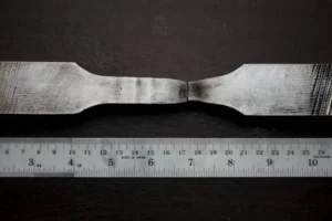
In a standard tensile test, we take a specimen (often a “dogbone” shaped metal coupon or a concrete cylinder) and gradually apply tension using a Universal Testing Machine. Initially, the material deforms elastically – meaning it will return to its original shape if the load is removed. As the load increases, the material may reach a yield point where it begins to deform plastically, i.e. permanent deformation that won’t recover on unloading. Pushing further, the material can strain harden (becoming stronger with deformation) until it hits the ultimate tensile strength (UTS) – the maximum stress the material can sustain. Beyond that, necking and eventual fracture occur.

Why is this curve so important? Because it encapsulates a material’s mechanical performance. Engineers use the stress-strain curve to determine if a material is suitable for a given application: for example, will it stretch too much under load? Will it break without warning? Does it have a high enough yield strength to carry expected forces? The curve provides answers by showing properties like Young’s modulus (stiffness), yield strength, tensile strength, and toughness (energy absorbed before breaking). Figure 1 below shows a typical stress-strain curve for a ductile metal (like mild steel) with these features labeled.

Figure 1: A typical engineering stress-strain curve for a ductile material (e.g. low-carbon steel). The curve starts with a linear elastic region (slope = Young’s modulus), then transitions at the yield point to the plastic region where permanent deformation occurs. It reaches a peak at the Ultimate Tensile Strength (UTS) and then eventually drops at the fracture point. Ductile materials like steel exhibit a noticeable plastic stretch before fracturing, whereas brittle materials would have a much shorter curve past yield.

Notice in Figure 1 how the steel sample first follows a straight line – that’s the elastic portion governed by Hooke’s Law (stress ∝ strain). The slope of this line is the Young’s modulus (E), which is a measure of stiffness. For instance, structural steel has a very steep slope (E ~ 200 GPa), indicating it’s very stiff, whereas a material like rubber has a gentle slope (low E, very stretchy). Up to the yield point, if you unloaded the steel, it would return to zero strain (no permanent damage). But beyond yield, the curve bends – the steel is now in the plastic regime and won’t fully return to its original length.

After yielding, the steel in this example shows a strain hardening region where the curve ascends again toward UTS. Strain hardening means the metal is gaining strength as it is deformed (due to mechanisms like dislocation interactions). Finally, after reaching the UTS, the engineering stress in the curve drops because the specimen begins to neck (thin down in a local region). Even though the actual stress in the neck (true stress) might still increase, the engineering stress (based on original area) falls until the material breaks apart at the fracture point.

In summary, the stress-strain curve is essentially the material’s fingerprint under load. Whether you’re a student testing a sample in the lab or an engineer simulating a structure in Abaqus, understanding this curve is crucial for predicting behavior. Next, we’ll learn how to interpret each part of the curve in detail.

How to Read a Stress-Strain Curve (Key Features)

Reading a stress-strain curve is like reading a story of how a material responds to force. Here are the key features and regions to look for on the graph, and what each tells you:

Axes Setup: The horizontal axis is strain (ε) – how much the material has deformed relative to its original length (it’s unitless, often expressed in percent). The vertical axis is stress (σ) – the applied force divided by the original cross-sectional area (units: Pa or N/m², often expressed in MPa for convenience). A point on the curve thus corresponds to “at this much deformation, the internal stress is this much.”

Initial Linear (Elastic) Region: The first portion of the curve is usually a straight line from the origin. This is the elastic region where stress and strain are proportional. The material obeys Hooke’s Law (σ = E·ε) and will return to its original shape if unloaded here. The slope of this line is Young’s Modulus (E), which quantifies the material’s stiffness. A steep slope (high E) means the material is very rigid (e.g. metals, ceramics), while a shallow slope means it’s flexible (e.g. polymers like rubber). For example, steel’s E ≈ 200 GPa, while concrete’s E is around 25–30 GPa, and polymers can be a few GPa or less – reflecting their relative stiffness.

Yield Point / Yield Strength: This is one of the most critical points on the curve. The yield point marks the transition from elastic to plastic behavior. On the graph, it’s often where the curve begins to deviate from a straight line and start curving or flattening. Up to yield, deformations are reversible; beyond yield, permanent deformation sets in. The stress at this point is called the yield strength (σ_y). For ductile metals like low-carbon steel, you may see a clear yield point where the curve even dips slightly (some steels have an upper yield and a lower yield plateau). However, for many materials (aluminum alloys, plastics, high-strength steel, etc.), there’s no obvious “kink” – the curve smoothly transitions. In those cases, engineers use the 0.2% offset method to define yield strength: essentially draw a line parallel to the elastic slope but starting at 0.002 strain (0.2%), and take its intersection with the curve as the yield point. This gives a convention for yield strength even when no clear drop is seen.

Plastic Region: After yielding, the curve enters the plastic region. Here, the material undergoes irreversible deformation. The curve often bends and becomes flatter than the elastic line, indicating the material still takes more strain with additional stress, but not as stiffly as before. In many ductile materials, you’ll observe strain hardening in this region – the curve may rise upward again after yield. This means the material is getting stronger as it is deformed; it requires increasing stress to continue plastically deforming. The physical reason is that the material’s internal structure (like the dislocation density in metals) is changing in a way that resists further deformation. The extent of strain hardening varies: mild steel, for example, has a significant strain hardening region, whereas a brittle material like cast iron or concrete might show almost none (they fail shortly after the elastic limit).

Ultimate Tensile Strength (UTS): This is the peak of the engineering stress-strain curve – the highest stress value reached. It’s also called ultimate strength. At this point, the material has developed as much internal stress as it can support. For a ductile metal under tension, after the UTS is reached, the phenomenon of necking occurs: the specimen’s cross-sectional area starts to significantly reduce in a localized region. Because engineering stress is calculated using the original area, once necking starts and the load bearing area shrinks, the engineering stress values on the curve begin to drop. It’s important to note that the true stress (based on actual reduced area) may still be increasing even as the engineering stress falls. But the UTS is a handy reference from the curve – it tells you the maximum load the material could handle before it started necking and heading toward failure.

Fracture (Breaking Point): The end of the stress-strain curve is the fracture point, where the material finally breaks into two pieces. At fracture, the stress abruptly drops to zero because the specimen can no longer carry load. The strain value at fracture is often taken as a measure of ductility – it’s the total elongation the material underwent before rupture. Ductile materials have a long elongation (the curve stretches far to the right), meaning they can deform a lot before breaking. Brittle materials have only a short extension – their curve ends quickly after yield. For example, a steel might endure 20% or more strain before breaking (especially if it necks a lot), whereas a brittle ceramic or concrete might fail at under 0.5% strain in tension. In a lab test, after fracture you can measure the pieces to find percent elongation and reduction in area, which are standard ductility metrics.

Young’s Modulus (Stiffness): As mentioned, this is obtained from the slope of the elastic region of the curve. It tells us how stiff the material is. Higher E means a small strain for a given stress (material resists stretching), while lower E means the material deflects more easily under load. Young’s modulus is an intrinsic material property used in design calculations – for example, to compute how much a beam will deflect under a load. It’s essentially the ratio σ/ε in the linear range. Some typical values: Steel ~ 200 GPa, Aluminum ~ 70 GPa, Concrete ~ 25 GPa (in compression), Polymers ~ 1–5 GPa (but rubber is in MPa range). Knowing E helps ensure structures remain within acceptable deformations under working loads.

Toughness (Area Under Curve): Toughness is a measure of how much energy a material can absorb before it fractures. On the stress-strain curve, it corresponds to the area under the entire curve (up to the point of fracture). A tough material requires a lot of energy input (work done by the force) to break it. Typically, strong and ductile materials are tough – they can take a lot of stress and also deform a lot, accumulating substantial energy. For example, structural steels are quite tough. On the other hand, a very strong but brittle material might have high strength but little deformation (small area under curve), so it would be classified as not tough. A classic comparison is steel vs. glass: steel can bend and absorb energy (tough), while glass, despite a decent strength, shatters suddenly with little energy absorption (brittle). Numerically, toughness can be quantified as modulus of toughness, the area under the σ-ε curve (often measured in units like MJ/m³). Engineers care about toughness for things like crashworthiness (how a material behaves in a car crash), impact resistance, and failure safety.

Ductility: This isn’t a single point but rather the extent of plastic deformation a material can undergo before breaking. On the curve, a long plastic region indicates high ductility. You can think of ductility as “how far to the right the curve goes.” It’s often reported as percent elongation at fracture or percent area reduction. Ductile materials (like mild steel, copper, many metals) will have a significant tail in the plastic region and visibly neck before breaking. Brittle materials (like glass, concrete in tension, cast iron) pretty much snap near the end of the elastic range – a very short or no plastic segment on the curve. Ductility is important for safety because a ductile material gives warning before failure (through visible deformation), whereas a brittle failure can be sudden and catastrophic. For example, reinforcing steel in concrete is ductile – if a structure is overloaded, the steel yields and stretches, giving large deflections that warn of trouble, rather than an abrupt collapse.

These key features make the stress-strain curve a rich source of information. By examining a material’s curve, you can quickly glean if it’s stiff or flexible (slope E), strong or weak (height of curve at UTS), ductile or brittle (length of curve before fracture), and tough or fragile (area under curve).

In the next sections, we will explore some of these aspects in more detail (like differences between materials, true vs engineering stress, etc.) and specifically relate them to common engineering materials steel and concrete.

Elastic Behavior and Young’s Modulus (Hooke’s Law)

When you first apply a small load to any solid material, it will typically deform in proportion to that load. This is the linear elastic behavior described by Hooke’s Law. In this regime, stress is directly proportional to strain and the constant of proportionality is the Young’s modulus (E). Mathematically:

which is a rearrangement of Hooke’s Law . This relationship holds up to the proportional limit (which for many materials coincides with the elastic limit or yield point).

Young’s Modulus (E) reflects the bonding strength between atoms in a material. Materials with strong atomic bonds (like metals with metallic bonds, or ceramics with ionic/covalent bonds) have high E, whereas polymers with flexible long-chain molecules have low E. For instance:

Metals: Steel ~ 200 GPa, Aluminum ~ 70 GPa, Copper ~ 110 GPa. These high values align with the rigid, tightly bonded crystal structures of metals.

Concrete: Around 25-40 GPa for typical concrete (exact value depends on mix and compressive strength). Concrete is a ceramic-like composite; its modulus is an order of magnitude lower than steel’s, which is why a concrete beam will deflect more than a steel beam under the same load.

Polymers: Polycarbonate ~ 2.5 GPa, Nylon ~ 3 GPa, and for contrast, a soft rubber might have E in the MPa range. That’s why plastics and rubbers are far more flexible.

It’s important to note that elastic strain is recoverable. If you remove the load while in the elastic regime, the stress returns to zero and the strain also goes back to zero – the material returns to its original dimensions exactly. In practical design, engineers often ensure that normal operating stresses stay below the yield strength, meaning structures generally deform elastically under service loads so that they don’t incur permanent set.

One more concept here is linear vs. non-linear elasticity: Most metals follow a nice linear Hookean behavior up to yield. However, some materials (like rubber) exhibit non-linear elasticity – the stress-strain curve is curved but still no permanent deformation occurs (this is typical of hyperelastic materials like elastomers). For our purposes, we focus on linear elastic solids which is the common case for metals and concrete up to initial cracking.

In summary, the elastic portion of the stress-strain curve is your material’s stiffness fingerprint. It tells you how much it will stretch under a given load, and it’s governed by the material’s Young’s modulus. A firm grasp of E is vital for everything from calculating deflections in buildings to selecting materials for springs or flexible joints.

Yielding and Yield Strength (When Elastic Turns Plastic)

The yield point is a pivotal moment on the stress-strain curve – it’s when the material “decides” that elastic time is over and plastic deformation begins. Up to the yield point, all deformation was temporary; beyond it, the deformation becomes permanent. This transition is hugely important in engineering design and analysis.

For many ductile metals (like mild steel), the yield point is quite evident. Mild steel famously shows an “upper yield point” followed by a small drop to a “lower yield point” and then a yield plateau. That appears as a little peak and dip in the curve around the yield stress. If you’ve seen a steel stress-strain chart, you might recall that flat-ish segment after the first yield drop – that’s the yield plateau where the material flows at roughly constant stress. During this phase, Lüders bands (deformation bands) can form and propagate along the steel sample while stress stays around the yield value. Once that plateau is passed, strain hardening kicks in and the stress starts rising again.

However, not all materials have a clear yield “kink.” Many do not. For example, aluminum and its alloys have a smooth curve – they gradually transition from elastic to plastic without a pronounced yield point. The same is true for a lot of stainless steels, some polymers, etc. How do we define yield strength in those cases? This is where the 0.2% offset yield method comes into play, as briefly mentioned earlier. Here’s how it works:

Take the initial straight-line portion of the curve (the elastic part) and determine its slope (E).

Starting at a strain of 0.002 (which is 0.2%), draw a line parallel to that initial slope.

The point where this offset line intersects the actual stress-strain curve is defined as the yield point by convention.

The stress corresponding to that intersection is reported as the yield strength (0.2% offset). Essentially, we’re saying “at this stress, the material has undergone a tiny 0.2% of permanent strain.” This standardized offset gives a consistent way to compare yield strengths across materials that lack a clear yield feature. When you see material property tables listing yield strength for aluminum, for instance, they were likely obtained by this method.

Why 0.2%? It’s somewhat arbitrary, but it’s a small strain that is usually imperceptible in practical use, yet beyond the typical proportional limit for many metals. It strikes a balance between being small enough to represent “nearly elastic” and large enough to measure reliably.

So what is happening inside the material at yield? On the microscopic level, this is when defects or dislocations in the material’s crystal structure start moving en masse. In metals, once the shear stress on certain slip planes is high enough, dislocations move and multiply, causing permanent shifts in the atomic arrangement – i.e., plastic strain. In yield of ductile metals, no cracks form yet; the material is just flowing plastically. In brittle materials, “yield” may correspond to the onset of micro-cracking instead (since they don’t have significant plastic flow – more on that in the next section).

From a design perspective, yield strength is often the most important number. We usually design structures so that working stresses never exceed yield. That’s because once you yield material in a structure, it will have permanent deformation – which might be unacceptable (think of a bent aircraft wing or a sagging floor beam). Yielding can also be a precursor to failure if it progresses. In safety-critical applications, a generous factor of safety is applied to yield strength to ensure elastic behavior under normal conditions.

However, there are cases where controlled yielding is actually desirable – for example, in earthquake-resistant design of buildings, steel frames are designed to yield in a ductile manner to dissipate energy (better to have some steel beams yield and absorb quake energy than to have a brittle sudden collapse). In such cases, understanding the yield behavior and post-yield strain capacity (ductility) of materials is crucial.

In summary, the yield point is the gateway from reversible to irreversible deformation. Knowing the yield strength of your material tells you the stress level to avoid for no permanent damage (or conversely, the stress level at which the material will start to permanently deform). It’s a cornerstone for material selection and structural design. Always respect the yield strength – Mother Nature doesn’t let you go back once you cross that line!

(Fun fact: The term “yield” is quite literal – the material is yielding or giving way. In the old days, some testing machines were called “extensometers” and operators would watch for the point where the needle suddenly moved a lot without much increase in load – indicating yield had been reached.)

Plastic Deformation and Strain Hardening

Once past the yield point, the material enters the plastic deformation regime. In this stage, each increment of strain is permanent. If you unload the material in the middle of plastic deformation, it will not trace back down the original path to zero; instead, you’ll be left with a residual strain (a permanent set). To visualize this, imagine a stretched plastic bag – remove the load and it doesn’t snap back to original size; it stays elongated.

In the plastic region, two important phenomena are usually observed in ductile materials: strain hardening and eventually necking (in tension tests).

Strain Hardening (Work Hardening): This refers to the increase in stress required to continue deforming the material plastically. On the stress-strain curve, strain hardening is seen as an upward slope after yield – the curve rises to a higher stress. What’s happening is that as the material’s crystal structure is deformed, defects (dislocations) multiply and interact, making further deformation more difficult. Essentially, the material is becoming stronger (harder) as it is worked – hence “work hardening.” For example, if you bend a paperclip (mild steel wire) back and forth, the bent part actually becomes harder and stronger than it was originally, due to strain hardening – though if you overdo it, it will eventually fracture from accumulated damage.

On our curve (Figure 1 earlier), after the initial yield and slight yield plateau, the rising portion up to the ultimate strength is the strain hardening region. During this phase, the metal is still supporting increasing stress with more strain. It may even regain some stiffness in the sense that if you unload it somewhere in the strain hardening zone, the unloading slope will be linear (parallel to the original elastic slope), and if you reloaded, it would yield again at a higher stress than the first time (because you’ve raised the yield point via hardening). This is how processes like cold working (rolling, drawing, etc.) strengthen metals: by plastically deforming them to introduce strain hardening, which elevates yield strength at the expense of ductility.

Not all materials exhibit much strain hardening. Brittle materials (like glass, ceramics, plain concrete) essentially don’t – they tend to fracture shortly after the elastic limit, with very little plastic flow. Some materials might even exhibit the opposite of hardening, called strain softening (for instance, some plastics after yield might require slightly less stress to continue deforming due to molecular alignment, or concrete in compression beyond peak stress softens as cracks form). But for most ductile metals, strain hardening is significant and is a useful property.

Ultimate Tensile Strength (UTS) and Necking: As strain hardening continues, the material’s load capacity reaches a maximum at the UTS. Beyond this point, for a ductile tensile test, the material starts to neck. Necking means the cross-sectional area of the specimen begins to localize and reduce significantly in one region. Since engineering stress = load / original area, once the load starts dropping (due to the reduced area and material instability), the curve goes downward. However, it’s interesting that in the actual necked region, the true stress (load / actual area at that instant) can still be increasing even as the overall load drops. In fact, if one were to convert an engineering stress-strain curve to a true stress-strain curve, you’d see the true stress curve rising continuously until fracture[8] (because true stress accounts for the shrinking area). But engineers typically work with the engineering curve for simplicity, and UTS is taken as the max engineering stress.

Necking indicates that the material can no longer sustain uniform elongation – all further elongation will be concentrated in that necked region until failure. The onset of necking can be predicted by Considère’s criterion (which basically says necking begins when the slope of the true stress-strain curve equals the true stress at that point). In practical terms, you’ll see the specimen thinning visibly at one section.

Fracture in the Plastic Regime: Finally, the material will fracture at the neck after reaching some final elongation. Ductile metals often show a characteristic “cup-and-cone” fracture surface under tension: one side looks like a cup and the other like a cone, indicating significant shear deformation at failure. This is a sign of ductility – lots of plastic movement happened before the final break. Brittle fractures, in contrast, are typically flat and perpendicular to the load, with little deformation.

It’s worth noting that when a material is unloaded from the plastic region (short of fracture), its unload path is elastic (slope = E) so the recovered strain is only the elastic portion. The difference between the total strain and recovered elastic strain is the plastic strain that remains. If reloaded, the curve will follow the unload-reload path up to the previous max stress, etc. This is relevant in cyclic loading, metal forming operations, and so forth.

In design, plastic deformation is sometimes allowed in controlled ways (like in beams under extreme loads or crash absorbers), but generally one has to be cautious because after plastic deformation the material has changed – often it’s stronger (due to hardening) but also less ductile. If something has yielded, repeated loading can lead to low-cycle fatigue or unexpected failure modes. That’s why designs try to stay in elastic, except for energy-absorbing members or deliberate plastic hinges.

To sum up: the plastic deformation stage is where the material shows its capacity for permanent change. Strain hardening gives it some added strength as a consolation for losing innocence (elasticity), up until the ultimate strength. Necking then marks the material’s surrender to localization, and fracture is the final chapter. Understanding this helps in fields like metal forming (where you want to maximize ductility and control hardening), structural engineering (ensuring ductile failure modes), and material science (developing alloys that have desirable hardening behavior).

Ductile vs. Brittle Materials (Steel vs. Concrete Behavior)

Materials can broadly be classified as ductile or brittle based on their stress-strain response. The difference lies in how much plastic deformation they can undergo before fracture, and the overall shape of their stress-strain curves. Let’s compare these behaviors, using steel (a ductile material) and concrete (a brittle material in tension) as prime examples:

Ductile Materials (e.g. structural steel, aluminum, copper): These materials have the characteristic long, drawn-out stress-strain curves with substantial plastic regions. They can sustain a lot of strain after yielding before they break. In a tensile test, a ductile metal will neck and elongate significantly. As a result, ductile materials tend to have high toughness – they absorb a lot of energy (area under curve) before fracturing[2]. Another hallmark is that ductile materials often have a fairly well-defined yield point (at least in steels) and then strain harden. Structural steel, for instance, yields around 250 MPa (for mild steel) and might have a UTS around 400–500 MPa, with 20–30% elongation at break in a standard test.

If you were to classify by percent elongation: ductile materials usually have > 5% elongation (many metals are 10–40%). They also typically show visible deformation before failure – a steel rod will neck down, wires will noticeably stretch, etc. In engineering, ductility is a desirable property in many applications because it means a component will yield and deform (giving warning or absorbing energy) rather than shatter suddenly. For example, steel reinforcement in concrete is ductile – it will yield and create large cracks (which are visible) before breaking, allowing structures to redistribute loads.

Brittle Materials (e.g. concrete, ceramics, glass, cast iron): These materials have very limited plastic deformation. Their stress-strain curves are short and steep – often essentially linear up until fracture. A typical brittle material might break at a strain of only 0.5% or less. For instance, a plain concrete cylinder in tension might crack at a strain of around 0.01–0.02% (tensile strength of concrete is very low), and even in compression, concrete’s peak strain is around 0.2–0.3% at maximum stress beyond which it softens and fails. Concrete is an interesting case: in compression it exhibits a sort of nonlinear curve that rises to a peak and then drops (because cracks form and it “softens”), but it doesn’t have a yield point or a long plastic flow – it basically goes from elastic to cracked and failing. In tension, concrete is brutally brittle – it cracks almost immediately when the tiny tensile strength is exceeded. In fact, for design purposes, engineers often assume zero tensile strength for concrete because it’s so brittle in tension.

Brittle materials usually do not show a clear yield point (the concept of yield is not very applicable, since there’s no significant plastic range). Instead, one might define “fracture strength” or use an ultimate strength which is basically also the breaking strength. They also tend to have lower toughness – they might be very strong (high stress at failure) but since strain is low, the energy absorbed is relatively small. A classic example: glass can have a very high tensile strength in theory (theoretical strength ~7 GPa), but it’s so brittle that any tiny flaw causes it to break at much lower stresses and without any plastic deformation.

One key difference in failure mode: ductile materials usually fail with a lot of deformation (e.g. a steel bar might neck to a point). Brittle failures are often sudden and catastrophic – the material snaps without warning. Think of a brittle failure as breaking a piece of chalk (just snaps) versus a ductile failure as bending a copper wire until it finally tears.

Let’s specifically contrast steel vs. concrete since the question emphasizes those:

Structural Steel: Ductile, with a prominent yield point, excellent tensile strength, and a long plastic region. Steel will yield and then harden. It’s also roughly equally strong in tension and compression (isotropic behavior). When it fails, it does so after appreciable necking (in tension) or yielding (in bending, etc.). This ductility allows steel structures to redistribute forces; if one part yields, load can flow to other members, avoiding immediate collapse.

Concrete: Brittle in tension (that’s why we reinforce it with steel to carry tension). In compression, concrete can withstand high stresses (e.g. 30 MPa or more for typical mixes, up to 100+ MPa for high-strength concrete), but it does not “yield” in a ductile way – it will crack and crush after a certain strain. Concrete’s stress-strain curve in compression starts linearly, then gradually curves to a peak at around 0.2% strain, and then drops off as the concrete softens due to microcracking. By about 0.3–0.4% strain, it’s failing. There’s no long tail of plastic flow – once peak is reached, failure is imminent. In tension, as mentioned, concrete basically cracks at ~5–10 MPa for normal concrete (which corresponds to an extremely small strain ~0.01%). So in design, we essentially treat concrete as having no tensile capacity (that role is given to steel rebar).

It’s interesting to note that reinforced concrete combines these behaviors: the concrete handles compressive loads (where it’s strong, though still brittle, but the steel confinement can give it some ductility in compression), and the steel bars handle tension (bringing ductility to the system). The result is a composite that is safer – steel yields and provides warning before ultimate failure, even as concrete might be crushing.

Another concept is fracture energy in brittle materials: in materials like concrete or rock, instead of toughness from a long plastic curve, we talk about fracture energy (energy to create a crack surface). It’s a different way to quantify brittleness.

To visualize the difference in curves: if you put a stress-strain curve of a mild steel and a concrete (in compression) on the same plot (normalized perhaps), steel’s curve would stretch far to the right with a clear yield and then a big plastic area, whereas concrete’s would go up and drop sharply with almost no “rightward” extension. A brittle material’s curve often looks almost like a triangle (straight line up and then down if plotted until failure), whereas a ductile material’s looks more like a rounded-off trapezoid or an elongated shape with a significant area.

Bottom line: Steel (ductile) and concrete (brittle) exemplify why engineers often pair them together – steel provides ductility and tensile strength, concrete provides compressive strength and stiffness. When designing or simulating these materials, one must use appropriate models: steel can be modeled with elastic-plastic material models that include yield and hardening, while concrete often requires fracture or damage models to capture its post-peak softening and cracking behavior.

From a stress-strain perspective, always be mindful of whether your material is expected to behave in a ductile or brittle manner, as it will dictate how you analyze safety. For ductile materials, the focus is on yield strength (since they will deform significantly before breaking, you ensure yield is beyond service loads). For brittle materials, the focus is often on ultimate strength and ensuring a high factor of safety (since there’s little warning before failure). Also, temperature and loading rate can change things: for example, steel at very low temperature can lose ductility and behave more brittle (as in the case of Liberty ships cracking in WWII – the steel became brittle in cold arctic waters). We’ll touch on such factors next.

True Stress vs. Engineering Stress

Throughout this discussion, we’ve been talking about the engineering stress-strain curve, which is the most commonly used version – stress calculated using the original cross-sectional area and strain using the original length. It’s simple and works well for most design purposes, especially when deformations are relatively small (or when we care about the initial yielding and up to UTS).

However, as hinted earlier, after necking begins, the engineering curve starts to deviate significantly from the actual material behavior because the geometry is changing a lot. This is where true stress and true strain come in:

Engineering Stress \sigma_{\text{eng}} = \frac{F}{A_0}

True Stress \sigma_{\text{true}} = \frac{F}{A_{\text{instant}}}
, where {A_{\text{instant}}} is the instantaneous (current) cross-sectional area under load.

Engineering Strain \varepsilon_{\text{eng}} = \frac{\Delta L}{L_0}
, based on original length.

True Strain \varepsilon_{\text{true}} = \ln\!\left(\frac{L_{\text{instant}}}{L_0}\right)
, effectively considering the continuous change in length.

For small strains, the difference between engineering and true measures is minor. But for large deformations, they diverge. Before necking, the main difference is that true strain is slightly larger than engineering strain for a given elongation (because of the logarithmic definition), and true stress is slightly higher than engineering (because area is reducing under Poisson’s effect even before necking). After necking, the differences become stark: as mentioned, engineering stress goes down after UTS, whereas true stress continues to rise until fracture. This is because in reality the material is still getting pulled harder in the neck – it’s just that the engineering calculation doesn’t account for the shrinking area.

Why do we care about true stress-strain? In material science and plasticity theory, true stress-strain is more fundamental. Many constitutive models (like those used in FEA for large deformation) use true stress-strain data to fit material behavior because they want to account for how the material continues to bear load even as it necks. For example, if you were to input a stress-strain curve into Abaqus for a metal going into large plastic deformation, you would typically convert the engineering data to true data and perhaps even extrapolate beyond necking using a model (since data after necking is not uniform anyway).

However, for the scope of this beginner’s guide: the main takeaway is to know that the engineering curve is a simplification. It’s perfectly fine up to the UTS and somewhat beyond, but it doesn’t tell the whole story post-necking. In design, we mostly care up to yielding or a bit beyond, so engineering values are used. But in simulations or forming operations, true stress-strain curves are needed for accuracy.

One interesting note: for most materials, if you convert the entire engineering curve to true terms, the true stress-strain curve will not show a drop at necking – it will typically keep rising smoothly (at least until very close to fracture). Also, in the uniform deformation region (before necking), the difference is just that true stress is higher than engineering stress because $A$ is smaller than $A_0$. There is a simple conversion for the uniform part:

These come from geometry assuming constant volume (plastic incompressibility in metals). After necking, the conversion is not so straightforward because the deformation is no longer uniform.

In summary, engineering vs true is about convenience vs accuracy for large deformations. Engineering stress-strain is convenient and sufficient for most structural engineering needs (and it’s what you directly measure in a simple tensile test output). True stress-strain is used in research and advanced analysis for capturing the material’s behavior under large deformation (like metal forming simulations). If you ever work with FEA software like Abaqus or ANSYS for plasticity, remember to use true stress-strain data for input – the software typically expects that, because it deals with deformation of the actual mesh (current configuration). In fact, Abaqus will automatically convert engineering to true if you check certain options, but it’s good to be aware.

For a beginner, the key point is: don’t be confused if you see two curves – just know one is the “engineering” representation (which we normally use in hand calculations and basic design) and the other is the “true” representation (which is used in more detailed analysis and captures that the material never actually lost strength up to fracture in a tensile test). Both start off identical in the elastic region, then diverge after significant plastic strain.

Effects of Temperature and Strain Rate on the Stress-Strain Curve

The stress-strain behavior of materials isn’t fixed in stone – it can change with external conditions. Two major factors that influence the curve are temperature and strain rate (how fast you deform the material). If you’ve ever noticed how a plastic becomes more flexible when heated or how taffy candy stretches differently if you pull it slowly vs jerk it quickly, you’ve seen these effects in action.

Temperature Effects: In general, raising the temperature tends to make materials more ductile and “softer” (lower yield strength, lower stiffness), while lowering the temperature makes materials stronger but more brittle. Essentially, heat gives atoms more energy to move past each other, so the material can deform more easily (yield at lower stress). For metals, increasing temperature usually reduces yield stress and UTS, and increases ductility (elongation to fracture goes up). At high enough temperatures, some metals transition from ductile to almost superplastic (very large elongations).

For example, structural steel at room temperature is tough and ductile. At a few hundred degrees Celsius (think of steel beams in a fire), its yield strength drops dramatically and Young’s modulus also drops – the steel can deform much more for the same stress (this is why steel structures can collapse in fires; the steel softens). Conversely, at very low temperatures (below 0°C and especially at cryogenic temps), some steels lose ductility and can become brittle. The classic case was the Titanic’s steel or WWII Liberty ships – the steel had a ductile-to-brittle transition temperature around the service conditions, so in the cold North Atlantic the steel hull could behave brittle and crack.

Polymers show an even more pronounced temperature effect: many have a glass transition temperature; below it they are glassy (hard and brittle), above it they become rubbery or ductile. For instance, a plastic ruler might snap if bent in a freezer, but the same will bend like rubber if heated.

Concrete, being a composite, also loses strength at high temperatures (plus water in it can cause internal spalling), and at low temperatures it doesn’t have much change except slight increase in strength (since colder concrete is a bit stronger in compression) but it’s brittle anyway.

Strain Rate Effects: Strain rate refers to how quickly you apply the deformation (strain) to the material. A higher strain rate (pulling very fast) tends to make materials effectively behave stronger and more brittle; a slow strain rate (pulling very slowly) tends to allow more ductility. Physically, at high strain rates, dislocations and molecular chains have less time to move/relax, so the material resists deformation more. Also, fast deformation can raise the temperature locally (from energy dissipated as heat), which can complicate things.

In metals, increasing strain rate typically raises the yield and tensile strength a bit. In steels, the effect is there but moderate for normal rates. In some materials like high-strength steels or certain alloys, the effect can be larger. For polymers, strain rate can drastically change behavior – pull some plastics slowly and they neck and draw, pull them fast and they might shatter. Rubber if pulled extremely fast can actually seem stiff (like throwing a rubber ball very fast at a wall, it can feel hard).

An everyday example: silly putty – if you pull it slowly, it stretches (ductile behavior), but yank it quickly and it breaks (brittle behavior). Same material, different strain rate.

Quantitatively, materials often have a strain rate sensitivity exponent or factor. For instance, an alloy might follow something like σ = K * (strain rate)^m, where m is small (like 0.02–0.2) for metals. High strain-rate loading such as impacts or explosions can significantly elevate the apparent strength of materials (also because inertial effects and the need to propagate cracks fast, etc., play a role).

Combined Effect – Temperature and Strain Rate: Interestingly, increasing temperature and increasing strain rate have opposite effects on yield strength. Higher temp lowers yield, higher strain rate raises yield. So they can counteract each other to some extent. This is why material testing specs often specify standard temperature (like 20°C) and strain rate (like 0.005 /s or something) for consistency.

In FEA simulations and material models, these effects can be included. For example, Abaqus allows temperature-dependent material properties and defines strain-rate dependent yield through something like the Johnson-Cook material model (commonly used for metals in impact simulations, which has terms for temp and rate).

For civil engineers working with steel or concrete, normal strain rates (like in building loads) are low, so we don’t typically worry about rate effects except in special cases (seismic loading is relatively fast, impact loads, etc.). Temperature effects are considered for fire engineering or cold climate considerations.

To summarize: higher temperature = more ductile, lower strength; lower temperature = less ductile (brittle), higher strength (until brittle fracture). Higher strain rate = higher strength, often less ductility; lower strain rate = lower strength, more ductility. These trends are general; actual numbers vary by material.

When conducting tests or using data, always note the conditions. And if you’re designing for extreme conditions (like a pressure vessel that sees low temperatures, or a car component in a crash – high strain rate), make sure to account for these factors in your material models. Our team has experience in simulating such conditions – for instance, we use material models that include strain-rate effects when analyzing automotive crash components or consider the temperature-dependent behavior of steel when assessing structures in fire.

How a Tensile Test is Conducted (From Lab to Curve)

You might be wondering, how do we actually get a stress-strain curve in practice? The answer is through a tensile test (for materials in tension) or analogous compression test for brittle materials like concrete. Let’s walk through a simple tensile test for a metal to illustrate the process:

Prepare a Standard Specimen: Typically, a test specimen is prepared with a specific geometry. For metals, this is often a “dog-bone” shaped sample – it has a narrow section in the middle (the gauge length) and wider ends so you can grip it. The narrow middle ensures the fracture will occur there, away from grips. The specimen’s original length $L_0$ (gauge length) and cross-sectional area $A_0$ are measured accurately.

Place in Testing Machine: The specimen is loaded into a Universal Testing Machine (UTM) or specifically a tensile testing machine. The machine has two grips – one fixed and one attached to a moving crosshead. The test will pull the grips apart at a controlled rate. An extensometer or strain gauge may be attached to the specimen to measure strain directly over the gauge length, especially for the elastic portion.

Apply Load and Record Data: The test begins by moving the crosshead, applying a tensile force on the specimen. The machine is equipped with a load cell to measure the force continuously. So as the test runs, we get readings of force and displacement (or strain). The crosshead speed can be set according to standards (commonly to achieve a certain strain rate like 0.005 mm/mm per minute in the elastic range, etc.). Modern machines are often run under strain control for metals (e.g., up to yield they control strain rate, after yield maybe switch to load control, etc., to capture data smoothly).

Elastic Region: Initially, as load increases, the extensometer shows strain increasing linearly with load. The machine’s software is plotting stress vs. strain in real time (stress = force/A0, strain = extension/L0). This part is usually uneventful – just a straight line. Operators often use this to calculate Young’s modulus.

Yield Point: At some stage, the material yields. If it’s a steel with a sharp yield, the load might even drop slightly or fluctuate (yield point phenomena). The curve on the screen would start to deviate from linear. If using an extensometer, sometimes at yield the strain may jump (so some standards require removing the extensometer at yield to avoid damage, and switch to crosshead displacement for further strain – which is less accurate but sufficient for large strains).

Plastic Region and Data Capture: As the test continues into plastic deformation, the machine keeps logging force and displacement. The stress-strain curve is drawn out. If the machine is displacement-controlled, it will keep elongating the specimen. You would notice the force maybe continuing to rise (strain hardening) until it reaches a maximum (the UTS). After UTS, if in displacement control, the force starts dropping (the machine is still pulling but the specimen is necking). The machine can have trouble post-necking because true strain localizes, but generally it can continue until break.

Fracture: Finally, the specimen breaks (typically in the middle of the gauge length for a properly done test). The machine records the final force drop. The test is stopped.

Post-Test Measurements: The broken pieces are taken out. The final length of the gauge section is measured (to get total elongation). The necked diameter (or thickness) at fracture is measured to get reduction in area. These give % elongation and % area reduction, which are reported ductility measures.

Processing Data: The raw data of force vs displacement is converted to engineering stress and strain using the initial dimensions. One can then plot the complete engineering stress-strain curve. Often, for the official report, yield strength is determined (if using 0.2% offset, a line is drawn or the data is analyzed to find the intersection). UTS is noted (max stress). Young’s modulus might be calculated from the initial slope. If needed, the data can be converted to true stress-strain (at least up to the uniform strain limit).

For concrete compression tests, a similar concept: use a hydraulic compression machine, measure load and displacement (or strain via compression platens or LVDTs). The stress = load / area (cross-section of cylinder), strain = change in length / original length. The curve will rise to a peak and then drop as the cylinder crushes (though in many standard compression tests, once the concrete starts to crush, the test ends since concrete fragments or the machine unloads when peak is passed).

For polymers, often a tensile test at controlled temperature (maybe with a temperature chamber if needed) is done, similar procedure. Some plastics neck and then draw (like yielding then the neck propagates along length at roughly constant stress – which gives a flat region in the curve as the neck travels).

Each material has testing standards (ASTM, ISO) that specify specimen shapes and test speeds to ensure consistency. For instance, mild steel might be tested per ASTM E8, concrete per ASTM C39 (for cylinders).

In an academic or industrial lab, these tests are routine to get material properties. In our EngineeringDownloads team, we often rely on such data to validate our simulation models. For example, when building an FEA model in Abaqus for a steel structure, we use tensile test data to define the plasticity of the steel. For concrete, we use compression test data to define the stress-strain curve in compression, and maybe a split-cylinder test for tensile strength, etc.

It’s quite fascinating to see the machine plot the curve live – for a ductile material you see that lovely peak and then the drop. And hearing the “pop” of the specimen breaking is the final ta-da of the test!

Understanding how the curve is obtained also helps you trust the data – it’s not just some theoretical thing; it’s empirical. And it has inherent variability: two tests on nominally the same material may give slightly different curves due to material heterogeneity, test speed, etc. Engineers account for that by using safety factors and statistical values (e.g., specifying yield strength as a minimum value that 95% of samples should exceed, etc.).

In summary, a stress-strain curve is born from a physical experiment where we pull (or compress) a sample in a controlled way and record how it stretches (or shortens) under load. It’s the most direct way to capture a material’s mechanical fingerprint. If you ever get a chance to do a tensile test in a lab, go for it – it will greatly solidify your understanding of these concepts when you see a piece of metal neck and break, and then match that to the curve plot.

Real-World Applications and Importance of the Stress-Strain Curve

The stress-strain curve might seem like a laboratory artifact, but its implications are everywhere in engineering and everyday life. Here are some real-world applications and examples where understanding and utilizing the stress-strain relationship is crucial:

Material Selection: Engineers use stress-strain data to choose appropriate materials for a given application. For instance, if you need to design a spring, you’d pick a material with a high yield strength and the ability to undergo many elastic cycles (perhaps a spring steel). If designing a biomedical implant, you might need a material with a certain stiffness to match bone (not too stiff, not too flexible) and enough toughness to not fracture – stress-strain curves of candidate materials (like titanium, stainless steel, cobalt-chrome alloys) are compared. The Young’s modulus tells you about deflection (for things like aircraft wings, you need a high E material like aluminum or carbon fiber so it doesn’t flex too much). The yield and UTS tell you how much load a part can handle. The elongation tells you if the material can be formed or bent during manufacturing without cracking (important for shaping operations).

Structural Engineering and Safety: Building codes and design standards rely on the properties obtained from stress-strain curves. For example, steel rebars in concrete must have a minimum yield strength (often 400 MPa or so) and a certain elongation percentage – this ensures ductility. Why do we insist on ductility? Because in events like earthquakes or overloads, a ductile failure (where steel yields) is far safer than a sudden brittle failure (which would be catastrophic). The stress-strain curve of reinforcement steel ensures that if a beam is overloaded, the steel yields (bends) giving a big warning (large deflections, cracking sounds, etc.) rather than the concrete suddenly shattering. In structural steel design (say for buildings or bridges), the yield strength (from the curve) is used to calculate the load the member can carry (with safety factors). During tests of new materials or when qualifying materials, engineers will often create stress-strain curves to verify that they meet the expected grade (for example, A36 steel should show a yield around 250 MPa and decent elongation).

Mechanical Design (Machines, Vehicles): When designing machine parts (gears, shafts, bolts), knowing the material’s stress-strain behavior is critical. Bolts, for example, are often tightened to a percentage of yield. Automotive engineers look at stress-strain curves to design car components that can absorb impact energy – for instance, the steel used in car crumple zones might be chosen for high toughness (area under curve) so it can deform and absorb crash energy. On the other hand, high-strength bolts might use a steel with a very high yield (perhaps 1000 MPa) but one that is still ductile enough to avoid brittle fracture. The trade-offs between strength and ductility are all evident in the stress-strain curve.

Aerospace Materials: In aircraft, where weight is critical, materials like aluminum alloys, titanium, and composites are used. Their stress-strain curves (especially the modulus and yield) determine how thin you can make a skin panel or how much load a wing spar carries. Composites don’t have a yield point per se (they’re more brittle), so design is done with ultimate strength divided by a safety factor, and by ensuring strains don’t exceed certain limits. The curves also inform fatigue design – e.g., staying in elastic range to avoid plastic deformation that could accelerate fatigue.

Academic Research and New Materials: When a new alloy or polymer is developed, one of the first things researchers do is run tensile (or compressive/torsional) tests to get stress-strain curves. This tells them how the material compares to existing ones – is it stronger? More ductile? For example, a new 3D-printed steel might be tested to ensure it has similar ductility to wrought steel. Researchers also use the curves to understand deformation mechanisms (the shape of the curve can hint at things like twinning, phase transformations, etc., in advanced materials).

Simulation and FEA Calibration: In finite element simulations (our specialty at EngineeringDownloads!), having an accurate stress-strain curve input is key to realistic results. For example, if we’re simulating a steel beam bending in Abaqus, we input the steel’s elastic modulus and a plasticity curve (yield point and strain hardening data). The simulation will then predict where yielding occurs and how much permanent deformation happens. Without a proper curve, the FEA might give wrong answers. Similarly for crash simulations of a car, the materials of each component are defined by curves so the software can calculate energy absorption and failure. We recently consulted on a project involving simulation of high-strength steel in an offshore structure – using the correct stress-strain curve (including the plateau and hardening) was vital to predicting how the structure would behave under extreme loads.

Quality Control: Manufacturers sometimes perform tensile tests on batches of material to ensure they meet specifications. If a batch of steel shows lower yield strength or less elongation than required, it might be rejected as it could be prone to brittle failure. The stress-strain test thus serves as a quality check. In concrete work, a form of stress-strain test (compressive strength test at 28 days) is done to make sure the concrete mix achieved the required strength.

Failure Analysis: When a component fails in service, examining its fracture surface and comparing against known stress-strain behavior can tell a tale. A very low elongation in a broken metal piece indicates a brittle fracture – maybe due to a flaw or the material being too cold or a wrong material used. Investigators will often infer from the mode of failure what might have gone wrong, e.g., “the steel experienced brittle fracture, whereas it should have yielded – perhaps the temperature was very low or the steel had an embrittlement issue.”

Extreme Events: The performance in accidents, earthquakes, etc., all ties back to stress-strain. For instance, during an earthquake, structural steel undergoes cycles of yielding – its ability to do so repeatedly without cracking (low-cycle fatigue) is related to the shape of its stress-strain hysteresis. Engineers design detailing (like beam-column connections) to ensure the steel can yield properly (forming plastic hinges) rather than the connection failing unexpectedly. This ductile design philosophy has saved many lives.

Biomedical Implants: Consider something like a hip implant or a bone plate – these are often made of titanium or stainless steel. Their stress-strain behavior should ideally be somewhat close to bone’s behavior in terms of stiffness (Young’s modulus) to avoid stress shielding (bone losing mass if the implant takes too much load). So materials are chosen not just for strength but for matching mechanical properties with the biological environment. If a material is too stiff, it might carry all the load and bone doesn’t get loaded, leading bone to weaken. So here the whole shape of the curve (and especially the elastic part) matters for compatibility.

As you can see, the humble stress-strain curve guides decisions in design, safety, and innovation across engineering disciplines. It’s why we spend so much time understanding it. When you see a skyscraper, a car, or even an iPhone shell, behind the scenes someone looked at stress-strain curves of materials to decide what could meet the demands.

In a nutshell: the stress-strain curve is the foundational data that bridges materials science and engineering practice. It informs us how far we can push a material and in what way it will fail if pushed too far. It’s a tool for making things safe and efficient. At EngineeringDownloads, whenever we tackle a simulation or a project, one of the first things we ensure is that we have the correct material curves in our models, because everything else (stresses, deflections, failures) flows from that.

Modeling Concrete and Steel Behavior in FEA (Abaqus, ANSYS, etc.)

Now that we’ve covered the theory of stress-strain curves, let’s talk about how we actually use this information in practical finite element analysis (FEA) software like Abaqus, ANSYS, or other FEM tools. This is where theory meets application. Our focus will be on modeling steel and concrete, since these are common structural materials with very different behaviors (ductile vs brittle), and the user specifically mentioned our software package for these.

Modeling Steel in FEA:

For structural steel or reinforcing steel, the stress-strain behavior can be input into FEA programs usually by defining an elastic modulus and a plasticity model. In Abaqus, for example, one common approach is to use an elastic-plastic material definition with isotropic hardening. You would specify: – Elastic: Young’s modulus E and Poisson’s ratio ν (this covers the initial linear region). – Plastic: A table of “yield stress” vs “plastic strain” values to define the plastic region. The first point might be (yield_strength, 0 plastic strain), and subsequent points give the stress at various plastic strains, effectively sketching the stress-strain curve beyond yield. Abaqus then connects your data points with straight lines to form the continuous plasticity curve.

Important: Abaqus (and most FEA) expects this plastic data in terms of true stress and plastic strain (with plastic strain meaning total strain minus elastic strain). If you provide engineering stress-strain, you need to convert it. Often for simplicity, if strains are not too large, one might input engineering values up to a point. But strictly speaking, for accuracy, convert to true stress-strain and then deduct the elastic part to get plastic strain values. Our EngineeringDownloads Steel & Concrete modeling package actually includes tools and tutorials on how to perform these conversions and input them correctly – ensuring your steel behavior in simulation matches the real curve.

For example, say we have a steel with yield at 250 MPa and UTS at 450 MPa at 20% strain (engineering). We would convert those to true values and input something like: Elastic: E = 210 GPa, ν = 0.3. Plastic table: – 250 MPa at 0 plastic strain (this indicates yield point), – perhaps 300 MPa at 5% plastic strain, – 400 MPa at 10% plastic strain, – 450 MPa at 15% plastic strain, – etc., until just before necking. (These numbers would come from the true curve.)

The software will then simulate yielding: when the von Mises stress in an element reaches 250 MPa, plastic deformation begins according to that curve. If your structure experiences stress beyond yield, Abaqus will redistribute loads as parts yield, just like a real structure would.

What about necking and failure? Standard plasticity models don’t simulate necking explicitly (necking will emerge from the model if the mesh can deform freely and if there’s any imperfection or localization). To simulate the actual fracture, you might need to include a damage or failure criterion. For steel, you might use something like a ductile damage model that triggers element deletion at a certain strain. Abaqus has options for damage based on fracture strain, etc. These require calibration (often from experiments). In many structural analyses, we don’t actually simulate the breaking in two; we go up to the point of heavy deformation. But in projects like crash simulation, yes, we include failure criteria.

Modeling Concrete in FEA:

Concrete is trickier because it’s not well-described by a single stress-strain curve in all conditions. It behaves differently in compression vs tension. In compression, it has an initial elastic part, then a nonlinear part up to peak, then softening. In tension, it basically cracks (brittle). FEA software address this via specialized material models.

Abaqus, for instance, provides the Concrete Damage Plasticity (CDP) model. This model allows you to input: – Elastic modulus and Poisson’s ratio. – Compressive stress-strain behavior (or yield in compression, including hardening and then softening). – Tensile behavior (usually tensile strength and a post-cracking damage curve to model how concrete loses capacity after cracking).

Using CDP, you can model concrete such that it will capture both the gradual failure in compression and the cracking in tension. You might input the uniaxial compressive stress-strain for concrete (maybe using an equation from a code or experiments – e.g., an initial linear up to ~0.2% strain at f_c, then descending branch). For tension, you input the tensile strength and a fracture energy or crack width parameter to define how it loses tension capacity after cracking (tension stiffening behavior).

Alternatively, in simpler analyses, concrete might be modeled as an elastic material until cracking, and then one might use discrete crack methods or simply not take tensile stress (for example, using rebar elements to carry tension).

Our Concrete modeling package at EngineeringDownloads provides step-by-step guidance on setting up these concrete material models in Abaqus. We cover how to derive the needed parameters (like dilation angle, fracture energy, etc.) and how to validate the model against known results. For instance, if you simulate a concrete cylinder, you should get a similar stress-strain response as measured in lab.

Steel Reinforcement in Concrete (Composite Modeling): Often, we model reinforced concrete by combining the concrete material model with embedded rebar (modeled as steel with an elastic-plastic curve). The rebar takes tension after concrete cracks. The stress-strain behavior of the rebar is input as described for steel. The interaction (bond) is usually assumed perfect in embedded region for simplicity.

Modeling Other Materials (just briefly): – In ANSYS, the approach is similar: define a multilinear isotropic hardening material for steel (with stress-strain points). For concrete, ANSYS has concrete material models (like the Concrete model based on Willam-Warnke or others) but often people use user-defined material if they want advanced behavior, or simply use an elastic with a crushable plasticity. – There are also material libraries and tools to help generate these curves. Some codes (like EN1992 for concrete) give formula for the stress-strain curve of concrete that one can directly implement. For steel, codes might assume an elastic-perfectly plastic or elastic-plastic with a certain hardening for simplicity in hand calcs, but in FEA you can use the full curve.

Calibration and Validation: When we set up a material model, we often simulate a test (like a single element in tension or a cylinder compression) to see if we get the correct stress-strain output. This is a good practice: if your input was correct, the “virtual test” should recreate the curve you expect. Our team routinely does this as a validation step.

Why advertise our package here? Because if you’re reading this and thinking “wow, there’s a lot to consider in simulating steel and concrete,” you’re right! That’s why we developed specialized Steel & Concrete FEM modeling packages at EngineeringDownloads. These provide ready-to-use tutorials, example simulation files, and consulting support to help you model things like a reinforced concrete beam in Abaqus or a steel frame connection, etc. We cover how to input the stress-strain curves properly, how to choose element types, how to apply loads, and interpret results. Essentially, we try to bridge the gap between theory (stress-strain in a book) and practice (stress-strain in a complex 3D FE model).

Example Application: Imagine you want to simulate a reinforced concrete beam bending until failure. You’d use concrete’s stress-strain in compression (so the top of beam can crush), steel’s stress-strain for rebars (so the bottom steel can yield in tension), and include a tensile cracking model for concrete so cracks form. When you run the simulation, you’d see initially linear behavior (both concrete and steel elastic), then steel yields (stress in steel hits yield, it starts to stretch more – you’d see the load-deflection curve soften), then concrete in compression might reach its crushing strain, eventually the beam fails (maybe by steel fracture or concrete crushing). The FEA outputs would correspond to this, and you could visualize regions of yielding and cracking. All that is driven by the material definitions we input, which come from those fundamental stress-strain curves and fracture properties.

In summary, FEA modeling of materials is essentially feeding the computer the stress-strain behavior (and additional failure criteria) so it can predict how a complex structure made of those materials will behave under load. Steel being ductile is relatively straightforward to model with plasticity. Concrete being brittle is more complex and often needs damage models. Our EngineeringDownloads team has deep expertise in setting up these models – we’ve helped clients simulate everything from steel-concrete composite columns to concrete slabs under blast loads, and a key part of that is getting the material behavior right. If you have a project or analysis involving such simulations, consider reaching out to us – we provide online consulting services to guide you through the process or even do the simulations for you, ensuring that your models are realistic and reliable.

(Quick tip: Always double-check units when inputting stress-strain data in any software! A common mistake is mixing up MPa vs Pa, or strain as % vs fraction. These errors can distort your material behavior in the simulation.)

Common Misconceptions about the Stress-Strain Curve

Before we conclude, let’s clear up a few misconceptions or pitfalls that often trip up beginners (and sometimes even experienced folks) when dealing with stress-strain curves:

Stress-Strain is not Load-Deflection: Sometimes newcomers see a load vs displacement graph from a test and think it’s the same as stress-strain. It’s not – at least not until you normalize by geometry. Stress-strain is a material property (intensive), whereas load-deflection is structural (extensive). You could have a long slender rod and a short fat rod of the same material – their load-deflection curves will differ (the long rod stretches more, the fat rod takes more load), but if you convert to stress-strain, both give the same curve (if material is same). So always distinguish material behavior from structural response.

Yield Point vs. Proportional Limit: Some assume the end of linearity is exactly the yield point. Often true, but not always. Some materials have a proportional limit that is a bit below the yield (slight deviation from linearity before full yield). Practically, they’re close, and we often use yield as the end of linear elastic. But just know that “elastic limit”, “proportional limit”, and “yield point” can be slightly different concepts in precise terms. For most engineering materials though, it’s fine to treat yield as the end of elastic behavior.

Hooke’s Law in Plastic Range: Once yielding happens, Hooke’s law (σ = E ε) no longer applies to total deformation. People sometimes confuse that. After yield, the relationship is nonlinear and you can’t use Young’s modulus to predict further strain. Hooke’s law only governs up to yield (or up to proportional limit). After that, we use plasticity theory. If unloading from plastic region, Hooke’s law does govern the elastic unloading part (with the same original E, assuming no damage).

Ultimate Strength is not the “breaking strength” for ductile materials: For ductile materials, UTS is the maximum engineering stress, which occurs at the onset of necking. The actual breaking (fracture) stress in engineering terms is lower than UTS (on the curve it drops). Some people misinterpret UTS as “the stress at which it breaks.” It’s actually a bit earlier than break. For brittle materials, effectively they break at UTS (since no necking). So context matters.

“Stronger material” vs “Tougher material”: It’s easy to think a higher stress curve (one that goes higher up) means “better”. But it depends on what you need. A high UTS but very brittle material (like high-carbon steel fully hardened) might be “strong” but not tough or ductile – it could shatter under impact or unpredictable loads. Sometimes a lower-strength but more ductile alloy is preferred for safety. Toughness (area under curve) and ductility (elongation) are as important as strength in many applications. For example, in earthquake design, a lower-strength steel with higher ductility is often preferred over a super high-strength brittle steel. Misconception is equating strength with “quality” universally – engineers must consider the whole curve.

Materials Always Behave as in the Textbook Curve: Real materials can have irregularities. For instance, the yield plateau in steel can have serrations (Portevin–Le Chatelier effect) in some alloys where the curve jerks due to dynamic strain aging. Polymers can have crazy curves that depend on temperature and rate (some have multiple yield points). Composite materials don’t have a single smooth curve – they might have multiple drops as fibers break. So the classic smooth stress-strain curve is the ideal for homogeneous isotropic materials, but actual behavior can be more complex. That’s not really a misconception but a caution: always look at actual test data for your specific material.

Poisson’s Ratio effect: Not directly about the curve itself, but sometimes forgotten – when a material is deformed, it usually also changes dimensions laterally. In elastic regime, the ratio of lateral strain to axial strain is Poisson’s ratio (ν). Most metals have ν ~ 0.3, rubbers ~ 0.5, concrete ~ 0.18. This doesn’t show up on the 1D stress-strain curve, but it’s an important part of material behavior. In FEA, you have to input ν along with E. If you see a volume change in what should be plastic incompressibility (like metals yielding at constant volume), it could be a misunderstanding of Poisson’s effect or using an inappropriate material model.

Stress above UTS? In a structural analysis using elastic design, one might calculate stress = force/area and get a value above the material’s UTS. Does that mean the component will experience that stress? In reality, no – if you try to push a material beyond its capacity, it will yield or fail; it won’t sustain a higher stress than its strength. So, when simplistic analysis gives a stress above yield or UTS, that just tells you your design is not okay (it will yield or break). The actual stress the material can hold is capped by its flow stress (plasticity or by failure). This is why in elastoplastic FEA, once yield is reached, stresses don’t just keep rising indefinitely; the structure deforms more at roughly yield stress until hardening allows some increase.

Concrete’s “curve” in tension is tiny: Newcomers might think concrete has a tensile stress-strain curve similar to compressive. But actually, concrete’s tensile curve is basically a line that ends at the cracking point (very small area). After that it’s not a curve but a post-crack behavior (carried by rebar or by some tension softening from aggregate interlock, etc.). So in analysis, don’t assign concrete a ductile tension behavior – it’s a brittle line. That’s why we reinforce it.

High Strength = High Stiffness? Some think if a material has high strength it must be “stiffer”. Not true – stiffness (modulus) and strength (yield/UTS) are not directly correlated. For example, a high-strength spring steel and a mild steel have roughly the same Young’s modulus (~200 GPa) even though one’s yield might be 300 MPa and the other 1000 MPa. Conversely, a low-strength rubber and a high-strength kevlar fiber – the kevlar is extremely stiff (high E) and strong, rubber is very flexible (low E) and weak, but you could also find materials like a silicone that’s low strength and low stiffness, or a high strength but moderate stiffness material, etc. Each property needs to be considered. The stress-strain curve gives you both: the slope (stiffness) and the heights (strength). But don’t conflate them. In materials like concrete vs steel: steel is both stronger and more deformable; concrete is weaker and stiffer in some ways (initial slope relative to ultimate strain).

Addressing these misconceptions helps ensure one doesn’t misuse the stress-strain data. We often clarify these points when teaching students or training engineers in our courses.

Conclusion

The stress-strain curve is truly a cornerstone concept for engineers. It distills a material’s mechanical performance into a simple graph, from which we extract critical design parameters: stiffness, yield strength, ductility, tensile strength, toughness, and more. Whether you are a civil engineer designing a safe building, a mechanical engineer designing a car axle, or a materials scientist developing a new alloy, the information in this curve guides your decisions.

In this guide, we explored the stress-strain curve in depth – starting from basic definitions of stress and strain, walking through the hallmark regions of the curve (elastic vs. plastic, yield point, strain hardening, necking, fracture), and highlighting differences between ductile and brittle materials like steel and concrete. We also touched on practical aspects like how temperature and strain rate affect material behavior, and how to actually incorporate these curves into simulations using FEA software.

For beginners, it’s normal if this feels like a lot of information. The key takeaways you should remember are: – Elastic region: Material behaves like a spring (Hooke’s law), defined by Young’s modulus. No permanent deformation here. – Yield point: The stress at which the material transitions to plastic behavior. Beyond this, it won’t fully return to original shape. – Plastic region: The material can deform significantly here (if ductile), absorbing energy. Strain hardening can occur, raising the stress needed to continue deforming. – Ultimate strength: The maximum engineering stress the material can support. After this, if it’s a ductile test, necking will occur. – Fracture point: Where the material finally breaks. Ductile materials have a large strain at this point, brittle materials have very little. – Ductile vs Brittle: Ductile materials (like structural steel) give you warning (yielding, large deformations) before failure. Brittle materials (like concrete in tension, cast iron) fail suddenly with little warning. Their curves reflect that (long vs short post-yield portion). – Use in design: Always ensure working stresses are below yield for safety (or design for controlled yielding if that’s the intent). Consider the whole curve for failure modes – not just strength but also how it fails (ductility/toughness). – Modeling in FEA: Input the correct material data (elastic and plastic where needed). For steel, it’s straightforward plastic curves. For concrete, use appropriate models for cracking/crushing. Verify your model reproduces known behavior.

As you move forward, you’ll see that virtually every advanced topic in mechanics ties back to the stress-strain response – be it buckling (which depends on material yielding), fatigue (which is influenced by how far into plasticity cycles go), or even thermal expansion (which couples with stress if expansion is restrained, related to elastic moduli).

Finally, a word from our team: At EngineeringDownloads, our mission is to help engineers and researchers bridge theory and practice. We offer specialized packages for modeling steel and concrete structures (as mentioned) and provide consulting services. If you have a challenging project – say, you need to simulate a complex reinforced concrete structure or you’re encountering difficulties with convergence in an Abaqus model due to material nonlinearity – our experts (including myself) are here to assist. We can help you set up material models correctly, interpret results, and even optimize designs using our knowledge of these material behaviors. The goal is to ensure that the simulations you run or the analyses you perform truly reflect real-world behavior.

Understanding the stress-strain curve is the first step toward mastering material modeling and structural analysis. We hope this guide has made the topic clear and approachable. Keep this knowledge handy, and you’ll find yourself using it constantly – from checking if a design will hold up, to explaining why a part failed, to deciding what material to use next.

Feel free to reach out to us at EngineeringDownloads for further training, simulation support, or consultation on your engineering projects. Here’s to building safe, efficient, and innovative engineering solutions – one stress-strain curve at a time!

Written by Saman Hosseini