Mastering Soil Modeling in FEA: A Practical Guide for Engineers

soil
Hosseini Saman
February 26, 2026
12 Minute

Introduction to Soil Modeling for Engineers

As engineers, we often encounter scenarios where structures interact directly with the ground. From foundations for high-rise buildings and bridges to pipeline integrity in challenging terrains, understanding how soil behaves under various loads is paramount. This is where soil modeling comes into play – translating complex soil characteristics into a format that can be analyzed using numerical methods like Finite Element Analysis (FEA).

Accurate soil modeling is critical for ensuring structural integrity, predicting settlement, assessing stability, and designing robust geotechnical solutions. Without it, our designs might be overly conservative (costly) or, worse, unsafe.

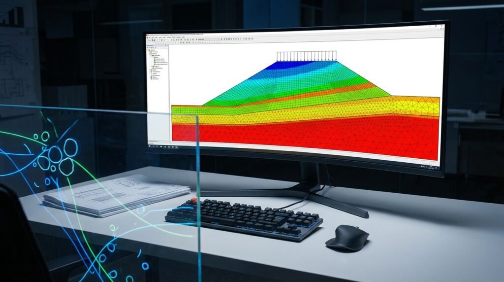
Image by Wikimedia Commons user Dr. J. T. St. Clair (USGS).

Why is Soil Modeling Challenging?

Unlike engineered materials like steel or concrete, soil is naturally heterogeneous, anisotropic, and exhibits highly non-linear, path-dependent behavior. Its properties are influenced by moisture content, density, stress history, particle shape, and geological formation. Capturing these complexities in a computational model requires a careful understanding of both soil mechanics and numerical analysis techniques.

Understanding Fundamental Soil Behavior

Before diving into FEA, let’s briefly recap key soil characteristics that influence modeling choices:

Non-linearity: Soil stiffness changes significantly with applied stress.
Plasticity: Permanent deformation occurs once yield stress is exceeded.
Path Dependency: The stress-strain response depends on the loading history (e.g., compaction, excavation).
Dilatancy: Volume changes during shearing.
Consolidation: Time-dependent volume change due to dissipation of pore water pressure.
Anisotropy: Properties vary with direction due to particle orientation or layering.

Key Constitutive Models for Soil Modeling

The core of soil modeling in FEA lies in selecting an appropriate constitutive model that mathematically describes the soil’s stress-strain relationship. Here’s a look at commonly used models:

1. Linear Elastic Model

Description: Simplest model, assumes linear stress-strain, elastic deformation, and no permanent strains. Uses Young’s Modulus (E) and Poisson’s Ratio (ν).
Use Case: Preliminary analyses, very small strains, or when soil behavior is dominated by elastic deformation. Often insufficient for realistic geotechnical problems.
Limitations: Ignores plasticity, shear strength, and volume changes under shear.

2. Mohr-Coulomb Model

Description: A classic elastoplastic model that defines failure based on shear strength, which is a function of cohesion (c) and angle of internal friction (φ).
Parameters: E, ν, c, φ, and often a dilatancy angle (ψ).
Use Case: Widely used for ultimate limit state analysis, slope stability, retaining walls, and foundations. Suitable for granular soils and normally consolidated clays.
Limitations: No strain hardening/softening, does not account for volumetric changes accurately, and can be overly stiff in some loading conditions.

3. Drucker-Prager Model

Description: A smoother, cone-shaped yield surface approximation of the Mohr-Coulomb criterion, often used to avoid numerical issues with the Mohr-Coulomb’s hexagonal yield surface.
Parameters: Similar to Mohr-Coulomb (cohesion, friction angle converted to Drucker-Prager parameters).
Use Case: Similar applications to Mohr-Coulomb, especially in dynamic analyses or situations requiring smooth yield surfaces for convergence.
Limitations: Shares many limitations with Mohr-Coulomb regarding volumetric behavior and path dependency.

4. Cam-Clay and Modified Cam-Clay Models

Description: Advanced elastoplastic models specifically developed for clays. They account for critical state behavior, hardening, and volumetric changes linked to shear deformation and mean effective stress.
Parameters: Critical state parameters (M, λ, κ), Poisson’s ratio, initial void ratio, and overconsolidation ratio.
Use Case: Essential for analyzing soft clays, consolidation, settlement, and liquefaction potential. Provides a more realistic representation of clay behavior.
Limitations: More complex parameter calibration; primarily for clays, not suitable for sands without modification.

5. Hypoplasticity Models

Description: A family of advanced constitutive models that aim to describe the continuous, non-linear stress-strain response of granular materials without explicitly defining an elastic domain or yield surface.
Parameters: A larger set of material constants calibrated from triaxial tests.
Use Case: Highly accurate for granular soils (sands, gravels) under complex loading paths, cyclic loading, and capturing phenomena like liquefaction.
Limitations: Significant computational cost, complex parameter calibration, and generally requires specialized knowledge.

Here’s a quick comparison of common soil models:

Model	Typical Use	Key Parameters	Complexity
Linear Elastic	Preliminary, very small strain	E, ν	Low
Mohr-Coulomb	Shear failure, granular soils, ultimate limit state	E, ν, c, φ, ψ	Medium
Drucker-Prager	Similar to Mohr-Coulomb, smoother yield surface	E, ν, Cohesion, Friction Angle (converted)	Medium
Modified Cam-Clay	Clays, consolidation, critical state behavior	M, λ, κ, ν, initial e, OCR	High

FEA Software for Geotechnical Analysis

Several commercial and open-source FEA packages offer robust capabilities for soil modeling:

Abaqus: Comprehensive material library, including Mohr-Coulomb, Drucker-Prager, Extended Drucker-Prager, and Modified Cam-Clay. Excellent for coupled pore-fluid diffusion and consolidation analyses.
ANSYS Mechanical: Features similar soil plasticity models. Can be integrated with other ANSYS tools for fluid-structure interaction (FSI) using Fluent/CFX.
Plaxis: A specialized geotechnical FEA software (by Bentley Systems) renowned for its advanced soil models, ease of use for geotechnical problems, and robust handling of consolidation and dynamic analysis.
OpenFOAM: Open-source CFD/CAE software that can be extended with custom soil models, though it requires significant user expertise.

Practical Workflow for Soil Simulations

Performing a soil simulation involves several critical steps. Follow this general workflow:

1. Geometry Definition and Meshing

Create Geometry: Accurately model the soil domain, including layers, geological features, and any structures interacting with the soil. Consider symmetry to reduce model size.
Mesh Generation: Use appropriate element types. For soil, often quadratic (second-order) elements (e.g., 8-node brick or 6-node wedge) are preferred for better accuracy in capturing non-linear behavior.
Mesh Density: Refine the mesh in areas of high stress gradients (e.g., near foundations, excavation edges) and coarser elsewhere. Consider aspect ratios, especially in thin layers or near contacts.

2. Material Property Assignment

Select Constitutive Model: Choose the most suitable model based on soil type, loading conditions, and desired accuracy (refer to the table above).
Input Parameters: Carefully obtain soil parameters from laboratory tests (triaxial, direct shear, oedometer) or reliable correlations. This is often the most critical and challenging step.
Layering: Define different material properties for distinct soil layers within your geometry.

3. Boundary Conditions and Loading

Displacement Constraints: Fix the base of the soil model in all directions. Fix vertical boundaries against horizontal movement but allow vertical displacement to avoid over-constraining. Ensure boundaries are far enough from the area of interest to minimize their influence.
Pore Pressure BCs: For consolidation or coupled analyses, define initial pore pressure conditions and drainage conditions (e.g., free draining, impermeable).
Applied Loads: Apply structural loads, distributed pressures, or imposed displacements as required. Consider the loading sequence (e.g., excavation followed by construction).

4. Analysis Steps and Solver Settings

Analysis Type: Static for immediate stability, transient for consolidation or time-dependent problems, dynamic for earthquake or impact analysis.
Non-linear Solution: Given soil’s non-linear nature, use an iterative solver with appropriate convergence criteria.
Load Stepping: Apply loads in increments, especially for highly non-linear problems. Automatic time stepping often helps convergence.
Convergence Criteria: Monitor force and displacement residuals. Adjust maximum iterations, damping, or arc-length methods if convergence is difficult.

5. Post-Processing and Interpretation

Deformation Plots: Visualize displacement, settlement, and strain fields.
Stress Contours: Examine effective stress, total stress, and pore pressure distributions.
Failure Zones: Identify regions where the soil has yielded or reached its failure criteria.
Reaction Forces: Check bearing capacities and structural interactions.

Verification & Sanity Checks for Soil Models

Robust verification is crucial to trust your simulation results. Here’s a checklist:

1. Mesh Sensitivity Analysis

Run the analysis with progressively finer meshes. Results (e.g., settlement, maximum stress) should converge to a stable value. If not, your mesh may be too coarse.

2. Boundary Condition Impact

Run a small sensitivity study by moving your model boundaries slightly further away. Verify that results in the region of interest do not significantly change, indicating your boundaries are sufficiently distant.
Check that prescribed boundary conditions (e.g., fixed displacements) are physically realistic for the problem.

3. Convergence Checks

Monitor the solver output for convergence warnings or errors. Non-convergence often points to highly non-linear behavior, poor mesh quality, or incorrect material parameters/boundary conditions.
For iterative solutions, ensure the force and moment residuals drop sufficiently, indicating equilibrium.

4. Validation (Where Possible)

Compare simulation results against analytical solutions for simplified cases, field measurements (e.g., inclinometer data, settlement gauges), or published experimental data.
Though often challenging, even approximate validation can significantly boost confidence.

5. Sensitivity Analysis of Material Parameters

Soil properties can have significant uncertainty. Perform runs by varying key parameters (e.g., cohesion, friction angle, stiffness) within a reasonable range (e.g., ±10-20%).
Understand which parameters have the most significant impact on your results, allowing for more informed design decisions or further site investigation.

Common Pitfalls and Troubleshooting

Incorrect Material Parameters: The most common source of error. Always prioritize quality geotechnical investigation data. Use appropriate correlations only when direct test data is unavailable and understand their limitations.
Poor Mesh Quality: Distorted elements or excessively coarse meshes in critical areas lead to inaccurate results or convergence issues. Prioritize a clean, well-structured mesh.
Non-Convergence: Often due to highly non-linear behavior, large load increments, or unrealistic material models. Try smaller load steps, adjust solver settings, or re-evaluate the constitutive model.
Over-simplification: Neglecting critical soil layers, geological features, or ignoring time-dependent effects (like consolidation) can lead to misleading results.
Ignoring Initial Stresses: For many geotechnical problems, defining an accurate initial stress state (geostatic stress) is crucial before applying additional loads.

Leveraging Automation in Soil Modeling

For repetitive tasks, parametric studies, or complex model setups, scripting can be a game-changer:

Python: Abaqus and ANSYS both have robust Python APIs for model generation, post-processing, and automation of analysis workflows.
MATLAB: Excellent for data processing, parameter calibration, and developing custom constitutive models before implementing them in FEA software.

If you’re looking to run larger, more complex soil models, consider EngineeringDownloads.com for affordable HPC rental, specialized online courses, internship-style training, or project consultancy to enhance your simulation capabilities.

Conclusion

Soil modeling in FEA is a powerful tool for geotechnical and structural engineers, enabling the design of safer and more efficient structures. By carefully selecting constitutive models, diligently preparing your FEA model, and rigorously verifying your results, you can confidently tackle complex soil-structure interaction challenges. Stay updated with advancements in constitutive modeling and computational geomechanics to continuously refine your practice.