S-N Curve Fatigue Analysis: Your Practical Engineering Guide

Fatigue
Hosseini Saman
February 27, 2026
16 Minute

Understanding S-N Curves for Fatigue Analysis: A Practical Guide

As engineers, we design components and structures to withstand various loads throughout their service life. While static strength is crucial, a far more insidious threat often lurks: fatigue. Fatigue failure can occur even when stresses are well below the material’s yield strength, making it a critical consideration in fields like aerospace, oil & gas, and structural engineering.

At the heart of understanding and predicting fatigue life lies the S-N curve, also known as the Wöhler curve. This practical guide will walk you through the fundamentals of S-N curves, their application in real-world engineering, and best practices for their use in your analysis workflows.

Image Credit: Cmglee, CC BY-SA 3.0, via Wikimedia Commons

What is an S-N Curve? The Basics

An S-N curve graphically represents the relationship between the magnitude of an alternating stress (S) and the number of cycles to failure (N) for a material under cyclic loading. Typically, stress amplitude is plotted on the y-axis (linear scale), and cycles to failure are plotted on the x-axis (logarithmic scale).

S (Stress Amplitude): This is usually half the range of the fluctuating stress. It’s the critical parameter dictating how quickly fatigue damage accumulates.
N (Number of Cycles to Failure): This represents the total number of load cycles a material can withstand at a given stress amplitude before it fractures due to fatigue.

The curve generally shows that as the stress amplitude decreases, the number of cycles to failure increases significantly. This inverse relationship is fundamental to fatigue design.

Key Concepts in S-N Curve Analysis

Endurance Limit (or Fatigue Limit)

For some materials, particularly ferrous alloys like steel, there’s a specific stress amplitude below which fatigue failure will theoretically never occur, regardless of the number of load cycles. This stress level is known as the endurance limit or fatigue limit. Materials like aluminum and copper alloys typically do not exhibit a distinct endurance limit; their S-N curves continue to trend downwards, meaning they will eventually fail given enough cycles, even at very low stress amplitudes.

Fatigue Strength

If a material does not have an endurance limit, or if you’re designing for a finite life, fatigue strength is the relevant term. Fatigue strength refers to the stress level a material can withstand for a specified number of cycles (e.g., 10^7 cycles) without failure.

Low Cycle vs. High Cycle Fatigue

Low Cycle Fatigue (LCF): Occurs at high stress amplitudes, often causing plastic deformation, and leads to failure in a relatively small number of cycles (typically less than 10^4 or 10^5 cycles). S-N curves can still be used, but strain-life (E-N) approaches are often more accurate for LCF.
High Cycle Fatigue (HCF): Occurs at lower stress amplitudes, primarily in the elastic range, and leads to failure after a large number of cycles (often above 10^5 cycles). S-N curves are the primary tool for HCF analysis.

Mean Stress Effects

The S-N curve is typically generated under fully reversed loading (mean stress = 0). However, most real-world applications involve a non-zero mean stress. A tensile mean stress generally reduces fatigue life, while a compressive mean stress can improve it. Engineers use mean stress correction models like Goodman, Gerber, or Soderberg diagrams to adjust S-N data for specific mean stress conditions.

Developing S-N Curves: Experimental Methods

S-N curves are primarily derived from experimental testing. Standardized tests, such as rotating bending or axial fatigue tests, involve subjecting multiple specimens of a material to various constant-amplitude cyclic stresses until failure. For each stress level, the number of cycles to failure is recorded. Due to the inherent scatter in fatigue results, statistical methods are used to interpret the data and often present S-N curves at different probabilities of survival (e.g., 50% or 95% survival rates).

Practical Workflow for S-N Curve Fatigue Analysis

Integrating S-N curves into your design and analysis process requires a systematic approach.

Data Collection & Material Characterization

The first step is acquiring reliable S-N data for the specific material you’re working with. This data can come from:

Material Handbooks and Standards: Industry-specific standards (e.g., for aerospace alloys, pressure vessel steels) often provide baseline S-N data.
Supplier Data: Material manufacturers may provide S-N data for their specific products.
Experimental Testing: For novel materials or critical applications, you may need to commission your own fatigue tests.

Crucially, ensure the S-N data corresponds to the material’s condition (heat treatment, surface finish) and environment (temperature, corrosive agents) relevant to your application. Generic data can lead to significant inaccuracies.

Stress Analysis (Analytical & FEA)

Once you have your material data, you need to determine the stresses your component will experience under cyclic loading.

Analytical Methods: For simple geometries and loading conditions, classical mechanics formulas can provide stress values.
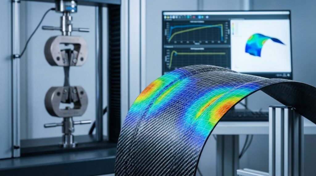
Finite Element Analysis (FEA): For complex geometries, stress concentrations, and multi-axial loading, FEA is indispensable. Tools like Abaqus, ANSYS Mechanical, and MSC Nastran allow detailed stress and strain distribution analysis. You’ll simulate the operational loads, paying close attention to peak stresses and stress gradients, especially at notches, fillets, and holes. These areas are prime locations for fatigue crack initiation.

Fatigue Life Estimation

With stress results and S-N data in hand, you can estimate the fatigue life:

Single Stress Amplitude: If your component experiences a constant stress amplitude, you simply read the corresponding cycles to failure directly from the S-N curve.
Variable Amplitude Loading (Cumulative Damage): Most real-world components experience varying stress amplitudes. Miner’s Rule (or Palmgren-Miner linear damage rule) is widely used to sum the damage caused by different stress levels:
- D = Σ (ni / Ni) where ni is the number of cycles applied at a specific stress level, and Ni is the cycles to failure from the S-N curve at that same stress level. Failure is predicted when D reaches 1.0.
Safety Factors: Apply appropriate safety factors to your estimated life or stress levels to account for uncertainties in material properties, loading, and manufacturing tolerances.

Integration with CAD-CAE Workflows

Modern engineering demands seamless integration. Your CAD models (e.g., from CATIA) feed directly into your CAE pre-processors. Post-processing tools, often enhanced with Python or MATLAB scripting, can automate the extraction of critical stress data, apply mean stress corrections, and perform cumulative damage calculations across numerous load cases. This automation is vital for iterative design and optimization, especially in areas like turbomachinery or biomechanical implant design.

Common Mistakes and Pitfalls

Ignoring Mean Stress: Assuming fully reversed loading when a significant mean stress exists can drastically overestimate fatigue life.
Using Generic S-N Data: Material properties vary. Using data for ‘steel’ when you need data for ‘normalized AISI 1045’ can lead to inaccurate predictions. Always match the material and its condition precisely.
Incorrect Stress Definition: Ensure you are using the correct stress amplitude (often peak-to-peak or alternating component) and considering stress concentrations accurately.
Extrapolating S-N Curves: Extending an S-N curve beyond its experimentally validated range can be highly risky.
Neglecting Surface Finish and Environment: Surface roughness, corrosion, or elevated temperatures can significantly degrade fatigue performance, effects not always captured by standard S-N curves.
Improper Mesh Refinement in FEA: Failure to adequately refine the mesh at stress concentration points will lead to inaccurate stress predictions and, consequently, flawed fatigue life estimations.

Verification & Sanity Checks in Fatigue Simulation

When performing fatigue analysis using FEA tools, rigorous verification and validation are non-negotiable for reliable results.

Mesh Quality & Refinement

Fatigue life is highly sensitive to local stresses. Ensure your mesh adequately captures geometry, especially in high-stress gradient regions (notches, holes, fillets). Perform a mesh convergence study to confirm that further mesh refinement does not significantly change the critical stress results.

Boundary Conditions & Loading

Carefully review your applied boundary conditions (BCs) and cyclic loading definitions. Do they accurately represent the real-world constraints and operational loads? Incorrect BCs are a common source of error. For dynamic loads, ensure the frequency and amplitude are correctly modeled.

Material Model Validation

Double-check that the material properties used in your FEA model, especially those related to elasticity and plasticity (if LCF is involved), are consistent with the S-N curve data source. Mismatched properties will invalidate your fatigue predictions.

Convergence Criteria

For non-linear FEA (e.g., involving plasticity), ensure your solution has converged adequately. Divergent or poorly converged solutions can produce wildly inaccurate stress fields, making any fatigue prediction useless.

Sensitivity Analysis

Explore how variations in key input parameters (e.g., material properties within their tolerance range, load magnitudes, boundary condition stiffness) affect your fatigue life predictions. This helps understand the robustness of your design and identify critical parameters.

Comparison with Analytical/Test Data

Whenever possible, validate your FEA results against simpler analytical models or, ideally, physical test data. Even a coarse correlation can boost confidence in your simulation methodology.

Factors Affecting Fatigue Life

Understanding these factors is crucial for effective fatigue design and analysis:

Factor	Description	Impact on Fatigue Life
Stress Amplitude	Magnitude of cyclic stress.	Higher stress = lower life. Primary driver.
Mean Stress	Average stress level in a cycle.	Tensile mean stress decreases life; compressive increases life.
Surface Finish	Roughness, residual stresses from manufacturing (e.g., machining, polishing).	Rougher surfaces (stress risers) = lower life. Shot peening can improve life.
Material Type & Treatment	Alloy composition, heat treatment, cold work.	Stronger, tougher materials with appropriate treatment generally have better fatigue resistance.
Temperature	Operating temperature.	Elevated temperatures often reduce fatigue strength due to creep-fatigue interaction.
Environment	Corrosive agents (e.g., saltwater), humidity.	Corrosion significantly accelerates crack initiation and propagation (corrosion fatigue).
Stress Concentrations	Geometric discontinuities (holes, fillets, welds).	High local stresses drastically reduce life; requires careful design and analysis.

S-N Curve Considerations for Specific Engineering Applications

Aerospace

Fatigue is paramount in aerospace. Aircraft components (wings, fuselages, landing gear) experience millions of load cycles. Designers often aim for ‘safe-life’ or ‘damage-tolerant’ designs. S-N curves are used extensively for material selection, component sizing, and defining inspection intervals. Python or MATLAB scripts are often employed to automate vast numbers of fatigue calculations for complex assemblies, considering factors like material anisotropy and fretting fatigue.

Oil & Gas

Offshore platforms, pipelines, and drilling equipment face harsh environments, variable wave loads, and corrosive conditions. S-N curves for welded joints are particularly critical here, often incorporating environmental factors. Fitness-for-Service (FFS Level 3) assessments frequently rely on fatigue crack growth analysis, which builds upon initial life estimations derived from S-N data.

Biomechanics

Designing prosthetics, implants, and medical devices requires understanding fatigue under physiological loading. Materials like titanium alloys and stainless steel are chosen for their biocompatibility and fatigue resistance. S-N curves help predict the lifespan of hip implants or dental devices subjected to millions of gait cycles or chewing forces.

Structural Engineering

Bridges, high-rise buildings, and other infrastructure components are subject to wind-induced vibrations, traffic loads, and seismic events. S-N curves for structural steel and concrete reinforcements guide design choices to prevent premature fatigue cracking, especially in connections and critical load-bearing elements.

Beyond S-N Curves: Other Fatigue Approaches

While S-N curves are fundamental, they are not the only tool. For different scenarios, engineers employ:

Strain-Life (E-N) Curves: More suitable for low cycle fatigue (LCF) where plastic deformation is significant, providing a more accurate representation of material behavior under high strain.
Fracture Mechanics (Paris Law): Focuses on the growth of existing cracks, predicting how quickly a crack will propagate under cyclic loading. This is crucial for damage-tolerant design and Fitness-for-Service assessments where initial defects are assumed or known.

Conclusion

S-N curve fatigue analysis is a cornerstone of reliable engineering design. By carefully characterizing materials, accurately determining operational stresses—often through advanced FEA tools like ANSYS or OpenFOAM for fluid-structure interaction—and applying sound fatigue estimation principles, engineers can predict component lifetimes and prevent catastrophic failures. Mastering this field is essential for ensuring structural integrity across diverse industries.

For more in-depth learning, specialized training, or high-performance computing (HPC) resources to run your complex fatigue models, explore the offerings at EngineeringDownloads.com, including online courses and consultancy services.

Frequently Asked Questions (FAQ)

Here are some common questions regarding S-N curves and fatigue analysis:

What is the primary purpose of an S-N curve in engineering?

The primary purpose of an S-N curve is to graphically represent a material’s fatigue resistance by showing the relationship between applied stress amplitude (S) and the number of cycles to failure (N). It helps engineers predict the lifespan of components under cyclic loading and design against fatigue failure.

Do all materials have an endurance limit?

No, not all materials exhibit a distinct endurance limit. Ferrous metals like steel typically have an endurance limit, a stress level below which they can theoretically withstand an infinite number of load cycles without failing. Non-ferrous metals like aluminum and copper alloys generally do not have a well-defined endurance limit; their S-N curves continuously decrease, meaning they will eventually fail given enough cycles, even at very low stresses.

How does mean stress affect fatigue life, and how is it accounted for?

Mean stress, the average stress in a cyclic load, significantly affects fatigue life. A tensile mean stress generally reduces fatigue life, while a compressive mean stress can extend it. Engineers account for mean stress effects using various correction models, such as the Goodman, Gerber, or Soderberg criteria, which modify the S-N curve based on the component’s specific mean stress conditions.

When should I use an S-N curve versus a Strain-Life (E-N) curve?

S-N curves are primarily used for High Cycle Fatigue (HCF) applications, where stresses are predominantly elastic, and failure occurs after a large number of cycles (typically > 10^5). Strain-Life (E-N) curves are more appropriate for Low Cycle Fatigue (LCF) applications, where stresses are high enough to cause significant plastic deformation, and failure occurs in a relatively small number of cycles (< 10^5). E-N curves better capture the material’s plastic strain response.

What are some common sources of error in S-N curve fatigue analysis?

Common sources of error include using generic or mismatched S-N material data, neglecting the effects of mean stress, overlooking surface finish and environmental factors (like corrosion), inaccurate stress calculations (especially at stress concentrations), and extrapolating S-N curves beyond their validated range. Poor FEA mesh quality in critical regions can also lead to highly inaccurate stress predictions.