In the world of engineering simulation, precision is paramount. Whether you’re designing a critical aerospace component, analyzing fluid flow in an oil pipeline, or assessing structural integrity, the accuracy of your models directly impacts the reliability and safety of your designs. One often-underestimated factor that can significantly compromise this accuracy is non-orthogonality.

At its core, non-orthogonality refers to situations where elements, surfaces, or coordinate axes are not perpendicular (orthogonal) to each other. While it might sound like a minor geometric detail, its implications in Finite Element Analysis (FEA), Computational Fluid Dynamics (CFD), and other simulation methods are profound, affecting everything from numerical stability to the trustworthiness of your results.

This article will demystify non-orthogonality, explaining where it arises, why it matters, and crucially, how engineers can identify, mitigate, and manage its effects in their daily simulation workflows. We’ll delve into practical strategies, tool-specific tips, and verification techniques to ensure your engineering analyses remain robust and accurate.

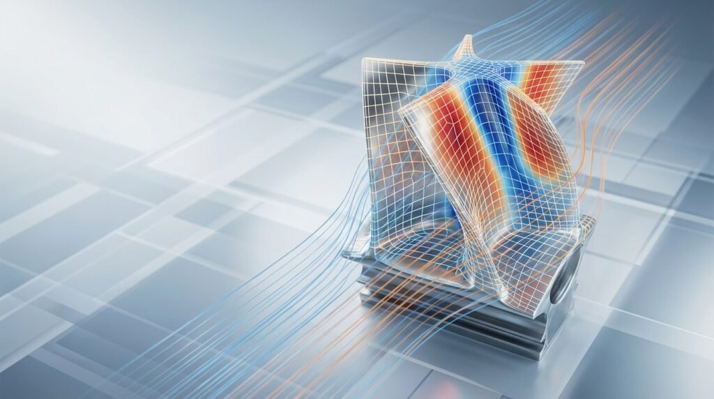
Image: Visual representation of mesh element quality, highlighting potential non-orthogonality through skewness.

What is Non-Orthogonality? A Practical Definition

Imagine a standard Cartesian coordinate system (X, Y, Z axes), where each axis is perfectly perpendicular to the others. This is an orthogonal system. Now, picture a situation where one axis is slightly skewed, forming an angle that’s not exactly 90 degrees with another. That’s non-orthogonality.

In engineering, this concept extends beyond simple coordinate systems to:

• Mesh Elements: In FEA or CFD, individual cells or elements in your computational mesh can be non-orthogonal if their faces or edges are not perpendicular to each other. This is often quantified by metrics like skewness, aspect ratio, or specific non-orthogonality measures.
• Geometric Features: Complex CAD models often contain angled surfaces, tapered sections, or intersecting features that are inherently non-orthogonal.
• Material Anisotropy: Materials with properties that vary with direction (e.g., composite laminates, wood grain) can be described using non-orthogonal material principal directions, requiring careful alignment with local coordinate systems.
• Loading/Boundary Conditions: Applying loads or boundary conditions at an angle to a surface’s normal vector can also introduce non-orthogonal considerations.

Why Does Non-Orthogonality Matter in Simulation?

The core issue is how numerical solvers handle these non-orthogonal situations. Most finite volume and finite element methods are formulated with an implicit assumption of orthogonal discretization or, at least, that non-orthogonality is minimal. When this assumption is violated, several problems can arise:

• Reduced Accuracy: The numerical approximation of gradients (e.g., stress gradients in FEA, velocity gradients in CFD) becomes less accurate, leading to erroneous results.
• Poor Convergence: Solvers struggle to reach a stable solution, requiring more iterations or even failing to converge altogether. This wastes computational time and can hide underlying issues.
• Numerical Instability: Solutions might oscillate or diverge, producing physically unrealistic results.
• Spurious Diffusion/Oscillations: Especially in CFD, non-orthogonal meshes can introduce artificial diffusion (smoothing out real flow features) or oscillations (creating non-physical wavy patterns).
• Increased Computational Cost: To compensate for poor element quality, solvers might need more sophisticated (and expensive) numerical schemes or finer meshes, increasing solution time.

Key Areas Where Non-Orthogonality Impacts Engineering Analysis

1. Meshing for FEA and Structural Integrity

In FEA, non-orthogonal elements are a significant concern, particularly with distorted elements like highly skewed quadrilaterals or tetrahedra. Poor mesh quality directly translates to inaccurate stiffness matrices and stress calculations.

Common Impacts in FEA:

• Stress Hotspots: Predicted stress concentrations might be exaggerated or understated, leading to incorrect assessment of structural integrity and potential failure.
• Stiffness Representation: Distorted elements may inaccurately represent the local stiffness, affecting overall structural response, deflection, and natural frequencies.
• Contact Analysis: Non-orthogonal element faces can complicate contact detection and pressure distribution, leading to convergence difficulties or inaccurate contact stresses.
• Fatigue & FFS (Fitness-for-Service): Inaccurate stress predictions from non-orthogonal meshes can lead to flawed fatigue life predictions or FFS Level 3 assessments, which are critical in Oil & Gas and Aerospace industries.

Tools and Metrics:

Software like Abaqus, ANSYS Mechanical, and MSC Nastran/Patran provide extensive mesh quality metrics. Key metrics related to non-orthogonality include:

• Skewness: Deviation of an element’s angles from the ideal (e.g., 90 degrees for quads/hexes, 60 degrees for equilateral tri/tet).
• Aspect Ratio: Ratio of the longest to the shortest edge length. While not strictly non-orthogonality, high aspect ratios in regions of steep gradients can exacerbate non-orthogonal effects.
• Jacobian Ratio: Measures the distortion of an element from its ideal shape.

Generally, aim for:

• Skewness: < 0.85 (for most applications, < 0.5 is excellent)
• Aspect Ratio: < 5-10 (depending on element type and application)

2. CFD and Fluid Dynamics Simulation

In CFD, non-orthogonal cells are notorious for causing numerical diffusion and convergence issues. Solvers like ANSYS Fluent/CFX and OpenFOAM are sensitive to mesh quality, especially near boundaries and in regions of high flow gradients.

Common Impacts in CFD:

• Artificial Diffusion: Non-orthogonal meshes tend to smooth out sharp gradients, masking critical flow features like vortices, shocks, or boundary layers.
• Discretization Errors: The approximation of convective and diffusive fluxes across cell faces becomes less accurate, introducing errors into the solution.
• Convergence Difficulties: Solvers may struggle to achieve residuals within acceptable limits, leading to prolonged simulation times or divergence.
• Poor Boundary Layer Resolution: Crucial for aerospace and turbomachinery applications, non-orthogonal cells near walls can severely impair the resolution of boundary layers, leading to inaccurate drag, lift, and heat transfer predictions.

Tools and Metrics:

CFD pre-processors (e.g., ANSYS Meshing, Pointwise, ICEM CFD) offer specific non-orthogonality metrics:

• Orthogonal Quality: A measure (typically 0-1) where 1 is perfect orthogonality. Values below 0.1-0.15 are often considered problematic.
• Skewness: Similar to FEA, but often with stricter limits for CFD (e.g., < 0.75 for general cells, < 0.25-0.5 for critical regions).
• Aspect Ratio: Critical for anisotropic meshes in boundary layers.

For most CFD applications, aim for an Orthogonal Quality > 0.15, ideally > 0.3.

3. Biomechanics and Anisotropic Materials

Biomechanics often deals with complex geometries (e.g., bones, soft tissues) and highly anisotropic materials (e.g., muscle, collagen fibers). Here, non-orthogonality can arise from both mesh quality and the definition of material properties.

• Complex Geometries: Generating high-quality meshes for patient-specific anatomies can be challenging, often resulting in non-orthogonal elements.
• Material Orientation: When defining anisotropic material models (e.g., in Abaqus or ANSYS), ensuring the material’s principal directions are correctly aligned with the local coordinate system and not inadvertently skewed is crucial.
• CAD Integration (CATIA, SolidWorks): Importing complex anatomical models from medical imaging (DICOM to CAD via tools like Mimics) often introduces geometric non-orthogonality that must be managed during meshing.

Practical Workflow for Managing Non-Orthogonality

Proactive management of non-orthogonality is key to successful simulations. Here’s a step-by-step workflow:

Step 1: CAD Clean-up and Simplification

1. Simplify Features: Remove small fillets, holes, or intricate details that are not critical to the analysis and would generate poor quality mesh.
2. De-feature: Use CAD tools (e.g., CATIA, SolidWorks, SpaceClaim) to remove unnecessary complexity.
3. Imprint/Split Surfaces: Where complex intersections occur, split surfaces to allow for structured meshing zones or better control over unstructured mesh transitions.
4. Identify Critical Regions: Know where high stresses, complex flows, or contact will occur, as these areas demand higher mesh quality.

Step 2: Intelligent Meshing Strategies

The mesh generation phase is where most non-orthogonality issues are introduced or resolved.

1. Global vs. Local Controls: Start with global mesh settings but apply local refinements and sizing controls in critical regions.
2. Structured Meshing (where possible): For simpler geometries or sub-domains, use mapped/structured hexahedral meshes (e.g., in ICEM CFD, ANSYS Meshing blocking) which inherently provide excellent orthogonality.
3. Unstructured Meshing with Care: For complex geometries, tetrahedral or polyhedral meshes are common. Polyhedral cells (available in Fluent, OpenFOAM) often offer better orthogonal quality than tetrahedra due to their multiple faces.
4. Pyramids/Prisms for Boundary Layers: Generate layers of high-aspect-ratio hexahedral/prismatic elements near walls to capture gradients accurately. Ensure the transition to the isotropic bulk mesh is smooth and orthogonal.
5. Mesh Smoothing/Optimization: Most meshing software includes algorithms to improve element quality. Use them iteratively, but always review the results as aggressive smoothing can sometimes distort elements in other ways.
6. Review Mesh Metrics: Always check orthogonal quality, skewness, aspect ratio, and Jacobian. Use visualization tools to locate problematic elements and refine locally.

Step 3: Solver Settings and Numerical Schemes

While mesh quality is paramount, solver settings can help mitigate the impact of residual non-orthogonality.

• Higher-Order Discretization: For CFD, higher-order schemes (e.g., second-order upwind) can improve accuracy on non-orthogonal meshes compared to first-order schemes, though they might also be less stable.
• Non-Orthogonal Correction: Many CFD solvers (Fluent, OpenFOAM) have explicit non-orthogonal correction schemes. Enable and tune these if your mesh has unavoidable non-orthogonality.
• Under-Relaxation Factors: In both FEA (for nonlinear problems) and CFD, judiciously reducing under-relaxation factors can improve convergence stability, especially with poor quality meshes, but at the cost of slower convergence.

Step 4: Post-Processing and Interpretation

Be aware that even with mitigation, residual non-orthogonality can influence results. When inspecting your solution:

• Identify Spurious Results: Look for unexpected oscillations, sudden jumps in scalar values (e.g., pressure, temperature), or unrealistic stress concentrations coinciding with poor mesh quality.
• Compare with Reference: If possible, compare results from a coarse, non-orthogonal mesh with a finer, higher-quality mesh in critical regions, or even analytical solutions.

Verification & Sanity Checks for Non-Orthogonal Effects

Never assume your simulation results are correct without thorough verification. Here’s a checklist:

Mesh Quality Audit:

1. Review the minimum orthogonal quality, maximum skewness, and maximum aspect ratio.
2. Visually inspect elements below thresholds in critical regions.
3. Perform local mesh refinement and re-run to see if results change significantly (mesh sensitivity study).

Convergence Behavior:

4. Monitor residuals closely. Are they dropping smoothly to acceptable levels?
5. Are mass, momentum, and energy balances satisfied?
6. Do solution variables (e.g., drag, lift, displacement, reaction forces) converge to a stable value?

Solution Sensitivity:

7. Grid Independence Study: Run simulations on several progressively finer meshes. If results change significantly between the finest two, your solution is still grid-dependent, potentially due to non-orthogonality.
8. Parameter Variation: Test slightly different solver settings (e.g., non-orthogonal correction schemes, under-relaxation) to see their impact on results and stability.

Physical Plausibility & Validation:

9. Do the results make physical sense? Are stresses in expected ranges? Is flow behavior realistic?
10. If experimental data or analytical solutions are available, compare your results.
11. For complex cases, consider a simplified benchmark problem with known non-orthogonal challenges to test your methodology.

Using Python & MATLAB for Automated Checks

For large projects or automated workflows, scripting can be invaluable:

• Mesh Quality Scripting: Python (with libraries like NumPy, SciPy) can be used to parse mesh files (e.g., from OpenFOAM or exported formats) and calculate custom mesh quality metrics, flagging problematic regions.
• Post-Processing Automation: MATLAB or Python can automate the extraction and comparison of results from different mesh refinements, helping with grid independence studies.
• Data Visualization: Generate custom plots and visualizations that highlight areas of poor orthogonal quality alongside solution variables.

Looking for custom scripts or advanced post-processing tools? Our online consultancy services can help develop tailored Python/MATLAB solutions for your specific simulation challenges.

Common Mistakes and Troubleshooting

Here are typical pitfalls and how to address them:

Mistake	Impact	Troubleshooting & Solution
Ignoring mesh quality reports.	Inaccurate results, poor convergence, wasted compute time.	Always review mesh quality metrics (orthogonal quality, skewness, aspect ratio) before running the solver. Address problematic areas with local refinement or mesh smoothing.
Over-relying on default solver settings.	Default settings might not be robust enough for non-orthogonal meshes, leading to divergence.	For CFD, enable non-orthogonal correction schemes. For both FEA/CFD, consider slightly lower under-relaxation factors initially, especially in nonlinear/transient problems.
Not performing a grid independence study.	Results might be highly dependent on mesh resolution and quality, masking non-orthogonality effects.	Always perform a grid independence study for critical parameters (e.g., drag, max stress, pressure drop) using at least three different mesh densities.
Aggressive mesh smoothing without review.	Can fix one quality issue but create others, or destroy important geometric features.	Use mesh smoothing iteratively and always inspect the resulting mesh quality and geometric representation. Manual clean-up or splitting geometry might be better than over-smoothing.
Using inappropriate element types for geometry.	Forcing hexahedral elements on highly complex, curved geometries can lead to severe distortion.	Consider polyhedral elements in CFD for complex regions, or switch to tetrahedrons/prisms for FEA. Embrace hybrid meshes (hex in structured regions, tet in complex).

Conclusion: Embracing Orthogonality for Robust Simulations

Non-orthogonality is an inherent challenge in complex engineering simulations, but it’s one that can be effectively managed with the right knowledge and tools. By understanding its causes and effects, adopting intelligent meshing strategies, leveraging solver capabilities, and performing rigorous verification, engineers can ensure their simulations yield accurate, reliable, and trustworthy results.

Prioritizing mesh quality, especially orthogonal quality, is not just a best practice; it’s a fundamental requirement for achieving robust and converged solutions in FEA, CFD, and other advanced analyses. By investing time upfront in CAD clean-up and mesh generation, you’ll save significant time and effort in debugging and re-running simulations later, leading to better designs and more confident engineering decisions.

Further Reading

ANSYS Blog: What is Orthogonal Quality?