Mastering Mesh Independence: An Essential Guide for Engineers

Meshing
Engineering Downlaods
March 20, 2026
12 Minute

In the world of computational engineering, especially within Finite Element Analysis (FEA) and Computational Fluid Dynamics (CFD), achieving accurate and reliable results is paramount. A crucial step often overlooked or incompletely performed is the Mesh Independence Study. This process ensures that your simulation results are not unduly influenced by the size or density of your computational mesh, providing confidence in your design decisions and analysis outcomes.

It’s about finding the ‘sweet spot’ where further mesh refinement yields negligible changes in your key results, thus balancing accuracy with computational cost. Without it, you might be analyzing mesh artifacts rather than true physical phenomena.

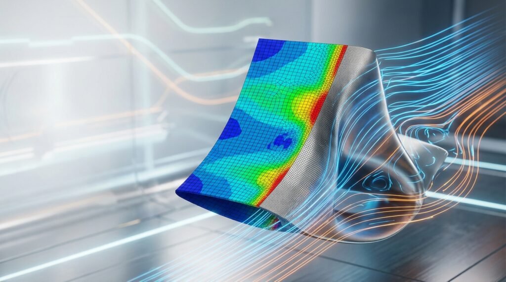
Image: Visual representation of mesh refinement around an airfoil.

Why is a Mesh Independence Study So Critical?

Performing a mesh independence study is more than just a ‘good practice’ – it’s fundamental for robust engineering analysis. Here’s why it matters:

1. Ensuring Accuracy and Reliability

True Physics vs. Numerical Artifacts: A mesh that is too coarse cannot adequately capture the intricate details of stress concentrations, flow gradients, or temperature distributions. Conversely, an overly fine mesh might introduce numerical noise or simply be overkill.
Trust in Results: For critical applications like structural integrity assessments (e.g., FFS Level 3 for Oil & Gas components) or aerospace designs, the reliability of simulation results directly impacts safety and performance.

2. Optimizing Computational Resources

Time is Money: Running simulations with excessively fine meshes consumes vast amounts of computational power and time. A mesh independence study helps identify the optimal mesh density, saving significant resources.
Project Efficiency: Efficient use of computational resources allows engineers to perform more design iterations, explore more scenarios, and deliver projects faster.

3. Validation and Verification (V&V)

Meeting Standards: Many industry standards and best practices for FEA/CFD (especially in fields like biomechanics or nuclear engineering) implicitly or explicitly require demonstration of mesh independence as part of the verification process.
Comparison Basis: When comparing your simulation results with experimental data or analytical solutions, ensuring mesh independence isolates potential discrepancies to modeling assumptions rather than meshing issues.

Understanding Mesh Quality and Its Impact

Before diving into refinement, it’s essential to understand what constitutes a ‘good’ mesh and how its quality influences your results.

Element Types

Tetrahedral (Tets): Versatile for complex geometries, but can be ‘stiffer’ in structural analysis if not properly handled. Often used for CFD volumetric meshes.
Hexahedral (Hexes): Preferred for structural analysis due to better accuracy and less sensitivity to distortion. Ideal for boundary layers in CFD.
Quadrilateral (Quads) and Triangular (Tris): 2D elements used for shell structures or surface meshing.

Key Mesh Quality Metrics

Software like Abaqus, ANSYS Mechanical, Fluent, and OpenFOAM provide tools to assess these metrics:

Aspect Ratio: Ratio of the longest edge to the shortest edge. High aspect ratios (e.g., >50 for boundary layers, >5 for general elements) can lead to poor accuracy.
Skewness: How close an element’s angles are to ideal (e.g., 90 degrees for quads/hexes, 60 degrees for tris/tets). High skewness degrades accuracy.
Orthogonality: For CFD, it measures how perpendicular face normals are to cell centroids. Low orthogonality impacts solution stability.
Jacobian Ratio: Measures the distortion of an element from its ideal shape. Values close to zero indicate severe distortion.
Growth Rate: How quickly element size changes from fine to coarse regions. Gradual changes are preferred to avoid numerical instability.

When Do You Need a Mesh Independence Study?

While often advisable, it’s particularly critical in specific scenarios:

New Geometries or Complex Loadings: Whenever you’re analyzing a novel design or intricate loading conditions that might induce localized effects.
Critical Design Analyses: For components where failure has severe consequences (e.g., structural components in aircraft, pressure vessels in Oil & Gas, prosthetic implants in Biomechanics).
High-Gradient Regions: Areas with rapidly changing stresses, temperatures, velocities, or pressures (e.g., crack tips, sharp corners, fluid boundary layers, heat sinks).
Transitioning from CAD to CAE: When using tools like CATIA or SolidWorks for design and then importing into CAE software, understanding how geometric features are represented by the mesh is vital.

Practical Workflow for a Mesh Independence Study

Follow these steps for a structured and effective mesh independence study:

Step 1: Define Objectives & Initial Setup

Identify Key Output Parameter(s): What are you trying to measure or predict? (e.g., maximum von Mises stress, peak displacement, lift/drag coefficient, pressure drop, heat transfer rate, reaction forces). This will be your convergence metric.
Establish Baseline Model: Create your initial FEA/CFD model, including geometry, material properties, boundary conditions, and loads. Start with a reasonably coarse mesh – not excessively coarse, but one that you expect to refine.

Step 2: Create a Series of Meshes

Generate at least 3-5 different mesh densities, ranging from coarse to progressively finer. Ensure systematic refinement.

Global Refinement: Simply reducing the global element size.
Local Refinement: Focusing refinement on critical areas identified in Step 1 or where you anticipate high gradients. This is often more efficient.
Boundary Layer Meshing: For CFD, ensure appropriate boundary layer elements (e.g., prism layers) are adequately refined, especially for turbulent flows (y+ considerations).

Step 3: Perform Simulations & Collect Data

Run your simulation for each mesh density using your chosen solver (e.g., Abaqus/Standard, ANSYS Fluent, MSC Nastran).
Extract the key output parameter(s) identified in Step 1 for each simulation.
Also record computational metrics like solve time and memory usage.

Illustrative Convergence Data Table

Mesh Density (Approx. Elements)	Max Von Mises Stress (MPa)	Max Displacement (mm)	Solve Time (min)
10,000	285.5	0.98	2
50,000	310.2	1.12	8
150,000	321.0	1.18	25
350,000	323.5	1.20	60
700,000	323.8	1.20	130

Step 4: Plot Results & Identify Convergence

Plot your key output parameter(s) against the number of elements (or a characteristic mesh size parameter).
Look for a point where the curve flattens out, indicating that further mesh refinement yields negligible change in the result. This is your convergence point. Typically, a change of less than 1-2% between successive refinements is considered converged.

Step 5: Determine Optimal Mesh Density

Select the coarsest mesh that lies within the converged region. This is your optimal mesh, balancing accuracy with computational efficiency.
Consider the trade-off: is the small gain in accuracy from a much finer mesh worth the significantly increased computational cost?

Step 6: Document Your Findings

Record your mesh convergence plots, chosen mesh density, and the rationale behind it. This documentation is crucial for verification and future reference.

Techniques for Mesh Refinement

Modern CAE tools offer various strategies to achieve good mesh quality and refine efficiently:

h-Refinement

This is the most common method, where you reduce the element size (h) in specific regions or globally. Most meshing tools (e.g., ANSYS Meshing, Patran, HyperMesh) allow you to control element size, density, and local refinement zones.

Adaptive Meshing

Some advanced solvers (e.g., Abaqus/Explicit, ANSYS Fluent) offer adaptive meshing capabilities:

h-Adaptivity: The solver automatically refines or coarsens the mesh based on error indicators during the solution process. This can be highly efficient for problems with moving boundaries or unknown high-gradient regions.
r-Adaptivity: Elements are moved to regions of interest without changing their number or connectivity.
p-Adaptivity: The polynomial order of the interpolation functions (p) is increased in elements without changing the mesh geometry. Less common for general-purpose studies but valuable in specific FEA contexts.

Common Mistakes and Troubleshooting

Even experienced engineers can encounter pitfalls during a mesh independence study:

1. Refining in the Wrong Areas

Mistake: Globally refining the entire model when only specific local regions (e.g., stress concentrations, fluid separation points) require finer meshes.
Troubleshooting: Perform an initial coarse analysis to identify high-gradient regions. Use local mesh controls or adaptive meshing.

2. Insufficient Refinement Steps

Mistake: Only testing two mesh densities (e.g., coarse and fine) which might not clearly show convergence or miss the optimal point.
Troubleshooting: Aim for at least 3-5 distinct mesh densities. Plotting the convergence curve is key.

3. Choosing an Inappropriate Convergence Metric

Mistake: Using a global average value (e.g., average displacement) when a local peak value (e.g., maximum stress at a hole) is the critical parameter.
Troubleshooting: Always choose a result parameter directly relevant to your design criteria and often a local maximum or minimum in a critical area.

4. Ignoring Mesh Quality Metrics

Mistake: Focusing solely on element count without checking element quality (aspect ratio, skewness). Poor quality elements can lead to inaccurate results regardless of density.
Troubleshooting: Regularly inspect mesh quality. Most software has tools to highlight problematic elements. If quality is poor, adjust meshing parameters or geometry clean-up.

5. Computational Cost Issues

Mistake: Refining so much that simulation times become prohibitive, especially for transient or non-linear analyses.
Troubleshooting: Prioritize local refinement. Consider parallel computing resources. If using Python or MATLAB for automation, optimize your scripts for efficiency.

Verification & Sanity Checks

Beyond the convergence curve, always perform these checks:

Visual Inspection: Look at stress contours, displacement plots, or flow streamlines. Do they make physical sense? Are there any unexpected localized ‘hot spots’ that might indicate mesh artifacts?
Conservation Laws: For CFD, check for conservation of mass, momentum, and energy. Any significant imbalance indicates an issue (often mesh-related).
Analytical/Simplified Models: Where possible, compare results from a coarse mesh to known analytical solutions or results from simpler models (e.g., beam theory for a structural component).
Boundary Condition Sensitivity: While not part of mesh independence, perform a separate sensitivity study on your boundary conditions and material properties to understand their impact.

Automation with Python & MATLAB

For repetitive or complex mesh independence studies, scripting can be a game-changer:

Scripted Mesh Generation: Tools like ANSYS APDL, Abaqus/Python scripting, or dedicated meshing APIs allow you to automate mesh creation with varying densities. This ensures consistency across different mesh models.
Automating Solver Runs: Python or MATLAB scripts can launch multiple simulation jobs, manage input files, and monitor their progress.
Post-processing & Plotting: Automate extraction of key results and generate convergence plots directly. This accelerates the analysis phase significantly.
CAD-CAE Workflows: Scripts can integrate with CAD tools (e.g., using Python for SolidWorks or CATIA APIs) to parameterize geometry before meshing and analysis, streamlining the entire design-to-simulation workflow.

For those tackling complex projects or seeking to optimize their CAD-CAE workflows, consider exploring our downloadable project templates or online tutoring services at EngineeringDownloads.com to help streamline your simulation processes.

Key Takeaways

Mesh independence is non-negotiable for reliable FEA and CFD results.
Systematically refine your mesh, especially in high-gradient regions.
Always plot your critical output parameter against mesh density to identify convergence.
Pay attention to mesh quality metrics, not just element count.
Leverage automation tools like Python and MATLAB for efficiency in complex studies.