Mastering Local Refinement in FEA & CFD Simulations

Local Refinement
Hosseini Saman
March 3, 2026
16 Minute

Understanding Local Refinement in Engineering Simulations

As engineers, we rely heavily on Finite Element Analysis (FEA) and Computational Fluid Dynamics (CFD) to predict structural behavior, fluid flow, and thermal performance. The accuracy of these simulations hinges significantly on the quality and density of the computational mesh. However, applying a globally fine mesh to an entire model is often computationally prohibitive and inefficient. This is where local refinement becomes an indispensable technique.

Local refinement is the strategic process of increasing mesh density only in specific, critical regions of a simulation model while maintaining a coarser mesh elsewhere. This targeted approach allows engineers to capture complex physical phenomena with high fidelity without incurring excessive computational costs or memory requirements. Whether you’re analyzing stress concentrations in a structural component or boundary layer development in fluid flow, mastering local refinement is key to obtaining reliable and efficient simulation results.

Image: Example of local mesh refinement around a hole in an FEA model. Image by T. E. Johnson, CC BY-SA 3.0, via Wikimedia Commons.

Why Local Refinement Matters: Critical Applications

The judicious application of local refinement is not just a best practice; it’s often a necessity for accurate engineering predictions across various domains. Here’s why:

Capturing Stress Concentrations in Structural Engineering

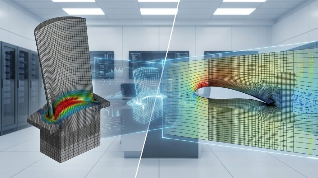
In structural integrity and FEA, regions with abrupt changes in geometry, such as fillets, holes, sharp corners, or notches, are prone to stress concentrations. Without sufficient mesh density in these areas, the peak stresses will be underestimated, potentially leading to unsafe designs or inaccurate fatigue life predictions. Local refinement ensures that these high-gradient stress fields are resolved accurately, which is vital for FFS Level 3 assessments in oil & gas and aerospace applications where safety margins are critical.

Resolving Boundary Layers in Fluid Dynamics (CFD)

For CFD simulations, accurately capturing the fluid’s behavior near solid walls is paramount. This region, known as the boundary layer, experiences steep velocity and pressure gradients. An insufficient mesh in the boundary layer can lead to incorrect drag, lift, heat transfer, and flow separation predictions. Local refinement, often through the use of ‘inflation layers’ or ‘prism layers’, builds high-aspect-ratio elements normal to the wall, providing the necessary resolution to capture these critical phenomena accurately, crucial for aerospace aerodynamics or turbomachinery design.

Accurate Contact Modeling

In FEA, especially for components undergoing contact (e.g., gears, bearings, bolted joints in structural assemblies), the contact surfaces require a fine mesh to accurately transfer loads and capture local deformations and stresses. Without it, contact pressures might be noisy, exhibit penetration, or simply be inaccurate. Local refinement ensures smooth contact interactions and robust convergence in simulations involving non-linear contact.

Addressing Fracture Mechanics and Crack Propagation

For advanced structural integrity analyses like fracture mechanics, understanding the stress intensity factors and crack growth rates requires extremely fine meshes around the crack tip. Specialized local refinement techniques, such as singular elements or highly graded meshes, are used to accurately resolve the stress field singularity at the crack tip, which is essential for predicting component life and failure in pipelines or aircraft structures.

Fundamentals of Local Mesh Refinement

Before diving into the practical steps, let’s clarify some core concepts.

What is Mesh Refinement?

Mesh refinement is the process of increasing the number of elements (and thus nodes) within a specific region of a computational domain. This leads to smaller element sizes, allowing the simulation to capture more detailed variations in physical quantities (e.g., stress, velocity, temperature).

Global vs. Local Refinement

Global Refinement: Involves reducing the average element size uniformly across the entire model. While it increases accuracy everywhere, it dramatically inflates computational cost, often unnecessarily, especially for large models.
Local Refinement: The strategic approach where mesh density is increased only in regions where high gradients or specific phenomena are expected, offering a balance between accuracy and computational efficiency.

Adaptive Mesh Refinement (AMR) – A More Advanced Approach

While this article focuses on static local refinement, it’s worth noting Adaptive Mesh Refinement (AMR). AMR is an advanced technique where the mesh automatically refines (and sometimes coarsens) during the solution process based on error indicators. Tools like ANSYS Fluent and OpenFOAM offer various AMR capabilities, providing even greater efficiency for transient or complex problems where critical regions might shift or evolve.

Practical Workflow for Local Refinement

Implementing local refinement effectively follows a structured approach within your CAD-CAE workflow. This workflow is applicable whether you’re using Abaqus, ANSYS Mechanical, Fluent, or OpenFOAM.

Step 1: Initial Mesh Generation and Baseline Simulation

Start with a Coarse Mesh: Begin with a relatively coarse global mesh that adequately represents the geometry but is quick to generate and solve. This provides an initial understanding of the model’s behavior.
Run a Baseline Simulation: Perform a preliminary simulation with this coarse mesh. This initial run helps identify areas of high gradients or critical behavior that will require refinement.

Step 2: Identify Critical Regions for Refinement

Based on your baseline simulation results and engineering judgment, pinpoint the exact locations needing refinement. This could be:

High-stress areas (FEA)
Contact interfaces (FEA)
Boundary layers and wakes (CFD)
Crack tips (FFS Level 3)
Regions of complex geometry or rapid solution changes

Step 3: Apply Refinement Techniques

Most commercial FEA/CFD software offers a range of tools to control mesh density locally.

Element Size Controls (General)

This is the most fundamental method. You can specify a desired element size for a specific:

Edge: For linear features (e.g., fillets, hole edges).
Face/Surface: For planar or curved surfaces.
Body/Region: For entire volumes (e.g., a specific component in an assembly).

In Abaqus, this is often done via ‘Seed Edges/Faces’ or ‘Assign Local Seeds’. In ANSYS Mechanical, you’ll find ‘Sizing’ controls for edges, faces, and bodies within the meshing branch.

Inflation Layers (CFD Specific)

For CFD, inflation layers (also known as prism layers or boundary layers) are crucial. These are layers of high-aspect-ratio hexahedral or wedge elements extruded from a wall surface into the fluid domain. They are specifically designed to resolve the steep gradients within the boundary layer. You typically control the first layer height, growth rate, and number of layers. ANSYS Fluent/CFX and OpenFOAM (via snappyHexMesh) provide robust controls for inflation layers.

Contact Sizing (FEA Specific)

In ANSYS Mechanical, ‘Contact Sizing’ allows you to refine the mesh specifically around contact pairs, ensuring better resolution and convergence at the interface. Abaqus users often apply local seeding to contact surfaces.

Body of Influence / Mesh Region (CFD/FEA)

Many tools allow you to define a ‘Body of Influence’ (ANSYS) or a ‘Mesh Region’ (Abaqus) – a non-physical geometric entity that acts as a zone for mesh refinement. Elements falling within this volume will be refined according to specified parameters. This is excellent for refining volumes around specific features without having to select individual faces or edges.

Python & MATLAB Automation for Meshing

For repetitive tasks or parametric studies involving meshing, scripting becomes invaluable. Tools like Abaqus offer a powerful Python scripting API for generating geometry, applying boundary conditions, and controlling mesh parameters programmatically. Similarly, ANSYS Mechanical can be driven by Python scripting (pyMAPDL) or APDL commands, while MATLAB can preprocess geometry or post-process mesh data. OpenFOAM’s snappyHexMesh utility relies heavily on dictionary-based configuration files, which can be generated or modified using Python scripts for automation.

Step 4: Iterative Refinement and Convergence

Local refinement is often an iterative process. Start with a moderate refinement, analyze results, and then further refine if necessary. The goal is to reach a mesh-independent solution, meaning further refinement does not significantly change the results of interest.

Common Tools and Their Approaches to Local Refinement

Here’s how some popular engineering simulation tools handle local mesh refinement:

Abaqus/CAE Meshing

Seed Edge/Face/Part: Direct control over element distribution along edges, on faces, or for entire parts.
Mesh Controls: Assign specific element types and meshing techniques (e.g., structured, swept, free) to regions.
Region Seeding: Specify global element sizes or biased element distributions for specific geometric regions.
Python Scripting: Advanced users leverage Python scripting to automate complex meshing strategies and parametric studies.

ANSYS Mechanical Meshing

Sizing: Apply element size controls to edges, faces, or bodies. You can define absolute sizes, number of divisions, or sphere of influence.
Inflation: Crucial for CFD and contact problems. Provides control over first layer height, growth rate, and number of layers along boundaries.
Body of Influence: Define a non-physical body to control mesh density within its volume.
Contact Sizing: Specific controls for refining mesh in the vicinity of contact pairs.

CFD Tools (Fluent, CFX, OpenFOAM)

ANSYS Fluent/CFX: Utilizes extensive meshing tools like ANSYS Meshing and SpaceClaim. Key features include inflation layers, body of influence, and source regions for refinement.
OpenFOAM (snappyHexMesh): A powerful block-mesher for complex geometries. It uses feature snapping and automatic cell splitting/refinement based on geometry, surfaces, and regions (refinementSurfaces, refinementRegions, featureEdges). This is highly scriptable and integrated into Python/MATLAB workflows for automation.

MSC Nastran/Patran

Mesh Seeding: Patran provides robust tools for seeding edges and surfaces, allowing engineers to specify mesh density and biasing.
Automatic Mesh Generation with Controls: Features like element sizing based on geometry features and global/local element size limits are available.

Verification & Sanity Checks for Refined Meshes

Simply refining the mesh isn’t enough; you must ensure the refined mesh is of high quality and that your results are physically sound.

Mesh Quality Metrics

Before running a solution, always check your mesh quality. Poor quality elements (e.g., highly distorted, high aspect ratio where not intended) can lead to inaccurate results or convergence issues. Common metrics include:

Metric	Description	Impact on Simulation
Aspect Ratio	Ratio of longest edge to shortest edge (or inscribed/circumscribed sphere radii).	High aspect ratio (e.g., >100 for FEA, >5 for CFD away from boundaries) can lead to numerical errors.
Skewness	Measure of how distorted an element is from an ideal shape (e.g., equilateral triangle, cube).	High skewness (e.g., >0.85 for tetra, >0.75 for hex) can reduce accuracy and stability.
Orthogonality	Angle between face normal and vector connecting cell centroids (CFD specific).	Low orthogonality (small angles) can introduce errors in flux calculations and lead to divergence.
Jacobian Ratio	Ratio of the largest to smallest determinant of the Jacobian matrix within an element.	Low values indicate element distortion, potentially leading to negative volumes.

Target values for these metrics can vary by solver and element type, but generally, lower skewness and aspect ratio (where appropriate) are better.

Boundary Condition Review

After refinement, double-check that your boundary conditions (BCs) and loads are still correctly applied to the newly refined mesh faces/nodes. Sometimes, selections can be inadvertently changed, or fine details might alter the application area.

Convergence Studies (h-Refinement)

This is arguably the most crucial check. Run simulations with progressively finer meshes in your critical regions. Plot the quantity of interest (e.g., peak stress, drag coefficient, natural frequency) against the number of elements or a characteristic element size. When the quantity of interest stabilizes and no longer changes significantly with further refinement, you have achieved mesh convergence. This is a form of h-refinement, where ‘h’ refers to the element size.

Solution Sensitivity Checks

Beyond mesh size, assess how sensitive your results are to other modeling choices (material properties, load application methods, contact parameters). This provides confidence in the robustness of your solution.

Comparison with Analytical or Experimental Data (Validation)

Whenever possible, compare your simulation results with known analytical solutions or experimental data. This validation step is the ultimate check of your model’s accuracy, including the meshing strategy.

Common Mistakes and Troubleshooting in Local Refinement

Even experienced engineers can stumble with local refinement. Here are common pitfalls and how to address them:

Over-Refinement

Mistake: Refining regions unnecessarily, leading to huge models, excessive computational time, and memory usage without a proportional increase in accuracy.
Troubleshooting: Perform convergence studies. If results don’t change after further refinement, you’ve likely over-refined. Focus refinement only where gradients are truly high or crucial to your design goal.

Insufficient Refinement

Mistake: Not refining enough, leading to inaccurate results, underestimated stresses, or failure to capture critical fluid phenomena.
Troubleshooting: Results often look ‘smooth’ but might be wrong. Check energy norms (FEA) or residual plots (CFD). High errors or residuals in critical regions indicate insufficient refinement. Always perform a convergence study.

Poor Element Transitions

Mistake: Abrupt changes in element size from fine to coarse regions can lead to distorted elements, inaccurate stress/flux transfers, and numerical noise.
Troubleshooting: Use smooth transitions, often achieved with geometric growth rates for element size. Most meshing tools have options for ‘growth rate’ or ‘bias factor’ to manage this automatically.

Refinement at Incorrect Locations

Mistake: Refining an area that is not critical, or missing a critical area altogether.
Troubleshooting: Use initial coarse mesh runs to identify high-gradient regions. Plot contour maps of stress, strain, velocity, or pressure to visually identify areas needing attention. Engineering judgment and prior experience are invaluable here.

Ignoring Mesh Quality Checks

Mistake: Proceeding with a solution without checking mesh quality metrics, especially after complex local refinement operations.
Troubleshooting: Always review mesh quality plots (skewness, aspect ratio, orthogonal quality) in your preprocessor. Isolate and fix bad elements if they occur in critical regions. Automatic mesh repair tools can help, but manual intervention might be necessary.

Best Practices Checklist for Local Refinement

Define Objectives: Clearly understand what results you need and which regions are most critical.
Start Simple: Begin with a coarse mesh to identify general trends and critical zones.
Iterate: Refine gradually and perform convergence studies.
Monitor Quality: Regularly check mesh quality metrics (skewness, aspect ratio, Jacobian).
Smooth Transitions: Ensure element size changes smoothly to avoid distortion.
Document: Keep records of your meshing strategy and convergence study results.
Automate: Use scripting (Python, MATLAB) for repeatable meshing tasks and parametric studies.
Leverage Resources: If you’re running complex, highly refined models, consider affordable HPC rental to speed up your computations. EngineeringDownloads.com also offers online/live courses and internship-style training to help you master these advanced simulation techniques, alongside project/contract consultancy for specific needs.