LES vs DES: Choosing the Right Turbulence Model for CFD

Turbulence
Hosseini Saman
March 3, 2026
14 Minute

Navigating Turbulence: LES vs. DES in CFD Simulations

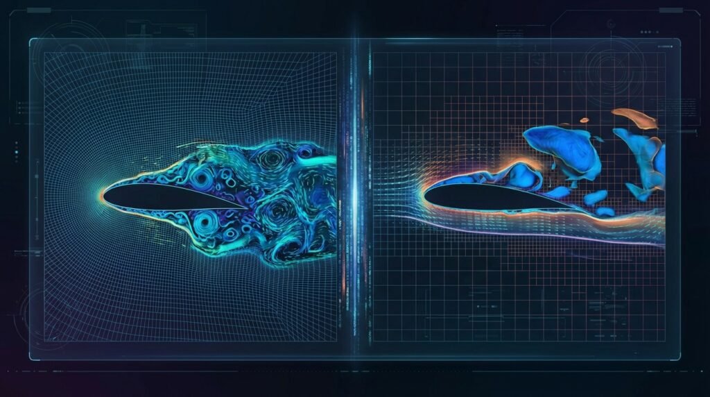
As engineers, we often encounter complex fluid flow phenomena where turbulence plays a critical role. From optimizing airfoil performance in aerospace to understanding mixing processes in oil & gas, accurate prediction of turbulent flows is paramount. While Reynolds-Averaged Navier-Stokes (RANS) models are workhorses for many industrial applications, they sometimes fall short when dealing with highly unsteady, separated, or anisotropic flows. This is where higher-fidelity models like Large Eddy Simulation (LES) and Detached Eddy Simulation (DES) come into play.

Choosing between LES and DES isn’t just a technical decision; it’s a strategic one that impacts accuracy, computational cost, and project timelines. This article will break down these two powerful turbulence modeling approaches, offering practical insights to help you make informed choices for your CFD projects.

Image: Turbulence visualization from a direct numerical simulation (DNS). Source: Kai Schneider via Wikimedia Commons.

Understanding Turbulence Modeling Fundamentals

Before diving into the specifics of LES and DES, let’s briefly recap why we need turbulence models at all. Direct Numerical Simulation (DNS), which resolves all scales of turbulence, is computationally prohibitive for most engineering problems due to its extreme mesh and time-step requirements. Turbulence models offer a way to approximate the effects of turbulence without resolving every minute detail.

The RANS Baseline: Strengths and Limitations

RANS models (like k-epsilon, k-omega SST) average the Navier-Stokes equations over time, making them computationally efficient. They model all turbulence scales, which is suitable for steady, attached, or mildly separating flows. However, they struggle with:

Highly unsteady flows (e.g., vortex shedding)
Massive flow separation (e.g., bluff body aerodynamics)
Flows with strong anisotropy or complex secondary flows
Acoustic predictions (due to averaging out transient fluctuations)

Large Eddy Simulation (LES): Resolving the Big Picture

LES takes a different approach. Instead of modeling all turbulent scales, it directly resolves the large, energy-containing eddies, which are typically anisotropic and geometry-dependent. The smaller, isotropic, and universal turbulent eddies are then modeled using a Sub-Grid Scale (SGS) model.

How LES Works

The core idea of LES is to apply a spatial filter to the Navier-Stokes equations. This filter separates the resolved scales (large eddies) from the sub-grid scales (small eddies). The large eddies are then computed directly, while the effects of the small eddies on the large ones are accounted for by an SGS model.

Key Characteristics of LES:

Resolution: Requires fine meshes to resolve large eddies, especially in critical regions.
Computational Cost: Significantly higher than RANS, as it’s a transient simulation and needs a much finer mesh and smaller time steps.
SGS Models: Common SGS models include Smagorinsky, Dynamic Smagorinsky, WALE (Wall-Adapting Local Eddy-viscosity), and Vreman models. The choice can influence results, with dynamic models generally being more robust.

When to Use LES: Ideal Applications

LES excels in scenarios where the unsteady behavior of turbulent structures is crucial. Consider using LES for:

Aeroacoustics: Noise generation from turbulent flows (e.g., aircraft landing gear, automotive mirrors).
Combustion: Detailed flame propagation, mixing, and pollutant formation.
Separated Flows: Bluff body aerodynamics, flow around complex geometries (e.g., risers in offshore oil & gas, biomechanical implants).
Mixing and Chemical Reactions: Understanding turbulent mixing processes in reactors or pipelines.
Heat Transfer: Where unsteady turbulent heat transfer is important.

Advantages of LES:

Higher accuracy for unsteady, separated, and highly anisotropic flows.
Provides detailed time-resolved flow fields, crucial for transient phenomena.
Less dependent on empiricism compared to RANS models.

Challenges with LES:

High Computational Cost: Demands substantial computational resources (HPC clusters).
Meshing Complexity: Requires very fine meshes, particularly near walls, which can be prohibitive.
Wall Modeling: Resolving the viscous sublayer directly (Wall-Resolved LES, WRLES) is extremely expensive. Wall Models (WMLES) are often used to reduce cost but introduce assumptions.

Detached Eddy Simulation (DES): The Hybrid Solution

DES is a hybrid turbulence modeling approach designed to combine the best aspects of RANS and LES. It uses a RANS model in the near-wall boundary layers, where RANS performs well and high resolution is needed, and switches to an LES formulation in detached, separated flow regions where large eddies dominate.

How DES Works

The transition between RANS and LES regions in DES is typically governed by a length scale, often based on the RANS model’s turbulent length scale and the local grid spacing. When the grid spacing is small enough (relative to the RANS length scale), the model behaves like LES; otherwise, it reverts to RANS.

Key Characteristics of DES:

Hybrid Approach: RANS near walls, LES in outer/separated regions.
Computational Cost: Lower than full LES, but higher than RANS.
Variants:
- DES: Original formulation, can suffer from “Model Stress Depletion” (MSD) or “Grid Induced Separation” (GIS) in certain conditions.
- DDES (Delayed Detached Eddy Simulation): Introduces a delaying function to prevent the LES part from activating too early in boundary layers.
- IDDES (Improved Delayed Detached Eddy Simulation): Further enhancements for robustness and consistency, especially for wall-modeled LES.

When to Use DES: Practical Applications

DES is a popular choice for industrial problems that require higher accuracy than RANS but cannot afford the full cost of LES. Ideal applications include:

Aerodynamics: High Reynolds number flows with significant separation, like automotive external aerodynamics, aircraft at high angles of attack.
Turbomachinery: Flow separation in compressors or turbines.
Offshore and Marine: Flow around structures, vortex-induced vibrations (VIV) in risers.
Internal Flows: Ducts with sharp bends, diffusers, or internal combustion engines with complex flow separation.

Advantages of DES:

Significant cost reduction compared to LES, especially for high Reynolds number wall-bounded flows.
Improved prediction of flow separation and reattachment over RANS.
More robust for industrial geometries than full LES.

Challenges with DES:

Grey Area Problem: The transition region between RANS and LES can sometimes introduce unphysical results or mesh dependency if not handled carefully.
Grid Dependency: Sensitivity to grid refinement in the LES region.
Still requires more computational resources than RANS.

LES vs. DES: A Direct Comparison for Engineers

To help you decide, let’s put LES and DES side-by-side on critical factors:

Feature	Large Eddy Simulation (LES)	Detached Eddy Simulation (DES)
Approach	Resolves large eddies, models small (sub-grid) eddies.	Hybrid: RANS near walls, LES in separated/outer regions.
Computational Cost	Very High (highest fidelity after DNS).	High (lower than LES, higher than RANS).
Meshing Complexity	Extremely high, especially near walls (WRLES).	High, but less demanding near walls than WRLES.
Near-Wall Treatment	Often uses Wall Models (WMLES) or very fine WRLES.	Uses RANS model near walls.
Accuracy for Unsteady Flows	Excellent, provides highly detailed transient data.	Good, especially for flows with significant separation.
Primary Use Cases	Aeroacoustics, combustion, detailed mixing, highly unsteady separated flows.	Industrial aerodynamics, turbomachinery, external flows with separation.
Typical Tools	ANSYS Fluent/CFX, OpenFOAM, Abaqus CFD.	ANSYS Fluent/CFX, OpenFOAM, Abaqus CFD.

Practical Workflow for LES/DES Simulations

Implementing LES or DES requires a meticulous approach. Here’s a typical workflow:

1. Problem Definition and Objectives

Clearly define what quantities you need to predict (e.g., pressure fluctuations, drag, heat transfer, mixing efficiency).
Understand the flow physics: Is it steady or inherently unsteady? Is separation expected?

2. Geometry Preparation (CAD-CAE Workflow)

Simplify complex CAD models (e.g., from CATIA, SolidWorks) to remove unnecessary details that won’t impact the flow.
Ensure clean geometry for meshing.

3. Meshing Strategies

Domain Extent: Ensure sufficient far-field boundaries to minimize artificial effects.
Mesh Type: Hybrid (prism layers near walls, polyhedral/tetrahedral elsewhere) or structured hexahedral meshes are common.
Wall Resolution:
- LES (WRLES): Aim for y+ < 1 for the first cell near the wall to resolve the viscous sublayer. This is very demanding.
- LES (WMLES): Use wall functions, y+ can be higher (e.g., 30-100), but careful validation is needed.
- DES: RANS region requires y+ < 1 or wall functions (y+ typically 30-100), LES region needs adequate resolution for large eddies.
Volume Mesh: Refine the mesh in regions of interest (e.g., shear layers, separation zones, wakes) where large eddies are expected.

4. Solver Setup

Turbulence Model: Select LES or DES (and its variant like DDES/IDDES).
SGS Model (for LES): Choose an appropriate SGS model (e.g., WALE, Dynamic Smagorinsky).
Time Step: This is critical. It must be small enough to resolve the fastest relevant turbulent eddies. A typical guideline is to ensure the Courant-Friedrichs-Lewy (CFL) number is less than 1, or even much less (e.g., 0.1-0.5) in critical regions.
Spatial Discretization: Use higher-order schemes (e.g., second-order central differencing) for convective terms to minimize numerical dissipation, which can dampen eddies.
Boundary Conditions: Define inlets (velocity profiles, turbulence intensity), outlets (pressure), walls (no-slip, temperature). Ensure physically realistic and stable BCs.

5. Simulation Execution

LES/DES simulations are typically run on High-Performance Computing (HPC) clusters due to their demanding nature. If you need robust and affordable HPC rental to run your large-scale CFD models, EngineeringDownloads.com offers specialized solutions.
Run an initial RANS solution to get a good starting flow field if convergence from scratch is difficult.
Run for sufficient physical time to capture statistical stationarity and relevant flow features.

6. Post-Processing

Analyze time-averaged quantities (mean velocity, pressure).
Analyze transient data: turbulent kinetic energy (TKE), Reynolds stresses, vorticity, pressure fluctuations.
Spectral analysis (e.g., Fast Fourier Transform – FFT) to identify dominant frequencies in unsteady phenomena.
Visualization of eddies, streamlines, isosurfaces.

Verification & Sanity Checks for High-Fidelity Simulations

Rigorous checks are essential to ensure the reliability of your LES/DES results.

1. Mesh Quality Assessment

Aspect Ratio, Skewness, Orthogonal Quality: Crucial for solution accuracy and stability. Ensure values are within recommended limits (e.g., orthogonal quality > 0.1).
Y+ Distribution: Verify that your y+ values are appropriate for your chosen model and wall treatment.
Mesh Sensitivity: Perform simulations on at least two different mesh densities (coarse and fine) to assess grid independence for key quantities.

2. Boundary Condition Checks

Flow Profiles: Verify inlet velocity, temperature, and turbulence profiles are correctly applied and physically consistent.
Recirculation: Ensure outlets are far enough from the region of interest to prevent recirculation affecting the main flow.

3. Time Step Sensitivity

Similar to mesh sensitivity, run simulations with at least two different time steps to confirm that key unsteady flow features are resolved and results are insensitive to further time step reduction.
Monitor CFL number throughout the domain.

4. Convergence Monitoring

Residuals: Ensure residuals drop several orders of magnitude. For unsteady simulations, residuals will often reach a cyclic state rather than a steady minimum.
Integral Quantities: Monitor key engineering quantities (e.g., drag, lift, pressure drop, mass flow rate at outlet) over time to ensure they reach a statistically stationary state.

5. Physical Consistency and Validation

Flow Direction and Patterns: Are the streamlines, pressure gradients, and velocity fields physically reasonable?
Energy Spectrum: For LES, verify that the energy spectrum shows a decaying inertial range (Kolmogorov -5/3 law) where the SGS model is active.
Comparison: Whenever possible, validate your simulation results against experimental data, analytical solutions, or higher-fidelity DNS data.

Common Pitfalls and Troubleshooting in LES/DES

Under-resolved Mesh: The most common issue. Leads to inaccurate turbulence prediction, excessive numerical diffusion, or unstable solutions. Symptoms: smooth, unrealistic flow features, incorrect TKE.
Too Large Time Step: Fails to capture transient physics, leading to instability or inaccurate results. Symptoms: numerical oscillations, divergence, or artificial smoothing.
Incorrect SGS Model (LES): Some SGS models may not be suitable for all flow types. Dynamic models often provide better universality.
Grey Area (DES): If the grid resolution in the RANS-LES transition region is inappropriate, it can lead to non-physical behavior. DDES/IDDES variants help mitigate this.
Initial Conditions: Poor initial conditions can delay convergence or lead to unphysical transients. A converged RANS solution is often a good start.
Boundary Condition Issues: Inlets with insufficient turbulence specification, or outlets too close to separation zones can significantly skew results.

Enhancing Your CFD Simulation Capabilities

Mastering advanced turbulence models like LES and DES takes practice and robust resources. EngineeringDownloads.com offers a range of services designed to empower engineers in this domain, including specialized online/live courses, internship-style training, and project/contract consultancy for complex CFD challenges. These resources can help you refine your skills in tools like ANSYS Fluent, OpenFOAM, and with scripting in Python or MATLAB for advanced post-processing.

Conclusion

Choosing between LES and DES is a critical decision in advanced CFD. LES offers the highest fidelity for unsteady, separated flows but comes with a hefty computational price tag. DES provides a pragmatic compromise, blending RANS efficiency with LES accuracy in regions of detachment. By understanding their underlying principles, practical workflows, and potential pitfalls, you can select the most appropriate model to achieve accurate, reliable, and cost-effective simulation results for your engineering challenges.