1. An Introduction to Non-Linear Continuum Mechanics

Finite deformation (also called large deformation or finite strain theory) is a framework in continuum mechanics that describes the behavior of materials undergoing significant volume changes, where strains and rotations are not small. Contrary to small deformation theories, which assume infinitesimal changes, finite deformation accounts for geometric non-linearities arising from large displacements, rotations, and stretches. This is vital in applications like rubber elasticity, metal forming, biomechanics (e.g., soft tissues), crash simulations, and polymer processing.

In finite deformation, the material’s configuration evolves from an initial (reference) configuration (undeformed state, often denoted as B0B_0B0​ or BrB_rBr​ in some references) to a current (deformed) configuration (BtB_tBt​). The motion is described by a mapping:

$$x=F(X,t)$$

where $X$ is a material point in the reference configuration, and $x$ is its position at time $t$.

Key motivations for finite deformation theory:

• Geometric non-linearity: Large rotations can make linear approximations invalid (e.g., a beam bending into a loop).

• Material non-linearity: Behaviors like hyperelasticity (e.g., Neo-Hookean, Mooney-Rivlin, Ogden models) or finite plasticity require strain measures that are objective (frame-invariant).

• Objectivity: Quantities must be independent of rigid-body motions, leading to concepts like objective stress rates.

2. A Contrast to Finite Deformation: Linear Formulation

To better comprehend the finite deformation, let’s briefly contrast it with the linear (infinitesimal) formulation, which is a simplification valid only for small deformations ($\text{strain}\ll 1$) and small rotations.

In linear theory:

• The displacement gradient is

\nabla u = \frac{\partial u_i}{\partial x_j}​​

where $u=x-X$ is the displacement vector.

• The infinitesimal strain tensor is the symmetric part:

ε=12(∇u+(∇u)T)\varepsilon = \tfrac{1}{2} \left( \nabla u + (\nabla u)^T \right)ε=21​(∇u+(∇u)T)

• The rotation tensor is the skew-symmetric part:

ω=12(∇u−(∇u)T)\omega = \tfrac{1}{2} \left( \nabla u – (\nabla u)^T \right)ω=21​(∇u−(∇u)T)

but rotations are neglected in strain measures.

Stress-Strain Relations in Linear vs. Finite Deformation

Stress-strain relations are linear, e.g., Hooke’s law:

$$\sigma =\mathbb{C}:\epsilon$$

where $\sigma$ is the Cauchy stress and $\mathbb{C}$ is the 4th-order elasticity tensor.

• The formulation uses the undeformed geometry for equilibrium (no distinction between reference and current configurations).

• Nonetheless, the linear formulation fails in large deformations because it does not account for changes in geometry (i.e., area/volume changes) or objective rates.

For instance, in Neo-Hookean work, linear theory cannot capture the volumetric locking or non-linear stiffening seen in finite strains. Finite deformation overcomes this by introducing non-linear kinematics and objective measures.

3. Key Kinematic Tensors in Finite Deformation

Finite deformation relies on tensors that describe the mapping between configurations. These are derived from the deformation mapping.

Deformation Gradient Tensor (F)

&
The deformation gradient is the fundamental tensor: a second-order tensor that maps infinitesimal line elements from reference to current configuration.

Properties of F:

:

• Determinant:

$$J=\det (F)$$

represents the volume ratio (change due to deformation). For incompressibility (e.g., in some Neo-Hookean models), $J=1$.

• Polar decomposition:

$$F=RU=VR$$

where $R$ is the orthogonal rotation tensor, $U$ (right stretch) and $V$ (left stretch) are symmetric positive-definite stretch tensors. This separates rotation from pure stretching.

• Strain measures derived from $F$:

C=FTF=U2(Right Cauchy–Green deformation tensor)C = F^T F = U^2 \quad \text{(Right Cauchy–Green deformation tensor)}C=FTF=U2(Right Cauchy–Green deformation tensor) E=12(C−I)(Green–Lagrange strain, a Lagrangian measure)E = \tfrac{1}{2} (C – I) \quad \text{(Green–Lagrange strain, a Lagrangian measure)}E=21​(C−I)(Green–Lagrange strain, a Lagrangian measure) B=FFT=V2(Left Cauchy–Green tensor)B = F F^T = V^2 \quad \text{(Left Cauchy–Green tensor)}B=FFT=V2(Left Cauchy–Green tensor) e=12(I−B−1)(Almansi strain, an Eulerian measure)e = \tfrac{1}{2} (I – B^{-1}) \quad \text{(Almansi strain, an Eulerian measure)}e=21​(I−B−1)(Almansi strain, an Eulerian measure)

• In hyperelasticity, the strain energy density is often a function of $C$ or invariants of $B$.

• In finite plasticity, $F$ undergoes multiplicative decomposition:

F=FeFpF = F^e F^pF=FeFp

separating elastic (FeF^eFe) and plastic (FpF^pFp) parts.

Velocity Gradient Tensor ($L$)

The velocity gradient is the spatial derivative of the velocity field v=x˙v = \dot{x}v=x˙:

L = \frac{\partial v_i}{\partial x_j}

It decomposes into:

• Symmetric part (rate-of-deformation tensor):

D=12(L+LT)D = \tfrac{1}{2} (L + L^T)D=21​(L+LT)

which describes the rate of straining.

• Skew-symmetric part (spin tensor):

W=12(L−LT)W = \tfrac{1}{2} (L – L^T)W=21​(L−LT)

which describes the rate of rotation (vorticity).

Also note:

L=F˙F−1L = \dot{F} F^{-1}L=F˙F−1

thus

D=12(F˙F−1+(F−TF˙T))D = \tfrac{1}{2} \left( \dot{F} F^{-1} + (F^{-T} \dot{F}^T) \right)D=21​(F˙F−1+(F−TF˙T)) W=12(F˙F−1−(F−TF˙T))W = \tfrac{1}{2} \left( \dot{F} F^{-1} – (F^{-T} \dot{F}^T) \right)W=21​(F˙F−1−(F−TF˙T))

Spin Tensor ($W$)

As mentioned, $W$ is the skew-symmetric part of $L$, representing the instantaneous angular velocity of material elements.

• It’s objective (unchanged under rigid rotations).

• It’s crucial for defining objective rates in non-linear mechanics.

• In hypoelastic models, stress rates are tied to $D$ and corrected by $W$ for objectivity.

4. Objective Stress Rates: Jaumann Rate of Cauchy Stress

Stresses in finite deformation must be objective to ensure invariance under superposed rigid motions.

• The Cauchy stress $\sigma$ (true stress in the current configuration) is objective.

• But its material time derivative σ˙\dot{\sigma}σ˙ is not, because it includes rotational effects.

The Jaumann rate (or Jaumann derivative) corrects this:

σJ=σ˙−Wσ+σW\sigma^J = \dot{\sigma} – W\sigma + \sigma WσJ=σ˙−Wσ+σW

This is a co-rotational rate, spinning with the material via $W$. It’s widely used in hypoelastic-plastic models, with:

σJ=C:D\sigma^J = \mathbb{C} : DσJ=C:D

for elastic response.

Other objective rates include:

• Green–Naghdi rate: Uses the rotation from polar decomposition $R$.

• Oldroyd rate: Useful in viscoelasticity.

• Truesdell rate: Accounts for volume changes.

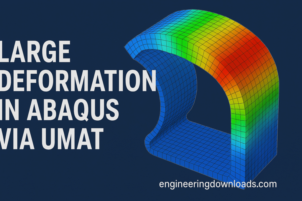
5. ABAQUS Implementation

In ABAQUS, finite deformation analysis accounts for geometric non-linearities by updating the geometry during simulation, using concepts like the deformation gradient, objective stress rates (e.g., Jaumann rate), and large-strain kinematics.

• When to Use It: Enable finite deformation when strains exceed 5% or when large rotations occur. It’s default for certain analyses (e.g., explicit dynamics in ABAQUS/Explicit) but must be explicitly activated in implicit solvers like ABAQUS/Standard.

• Key Feature: The *NLGEOM (Non-Linear Geometry) option toggles finite strain formulation. When ON, ABAQUS uses updated Lagrangian or total Lagrangian approaches internally, computing quantities like Green–Lagrange strains and 2nd Piola–Kirchhoff stresses.

• Advanced Modeling: The user subroutine UMAT allows for advanced implementations.

5.1. Setting Up a Finite Deformation Analysis in ABAQUS

Step 1: Model Creation and Geometry

• Create or import your geometry in ABAQUS/CAE.

• Assign sections: Define material properties and element types early, as finite deformation requires compatible elements.

Step 2: Material Models for Finite Deformation
ABAQUS supports various constitutive models that inherently handle finite strains:

• Hyperelasticity: Use *HYPERELASTIC.

• Plasticity: Use *PLASTIC with *HARDENING for finite strain plasticity (multiplicative decomposition).

• Viscoelasticity / Hyperfoam: For time-dependent or porous materials.

• Custom Models: Use UMAT or VUMAT (Explicit) to define constitutive equations, incorporating deformation gradient, velocity gradient, and spin.

Tip: For incompressible materials ($J\approx 1$), enable hybrid elements to avoid locking.

Step 3: Element Selection
Choose elements that support finite strains:

• Solid Elements: e.g., C3D8R for 3D, CPE4R for 2D plane strain.

• Shell/Beam: e.g., S4R for shells under large rotations.

• Hybrid Elements: Add H suffix (e.g., C3D8RH) for nearly incompressible cases.

Step 4: Step Definition and Enabling Finite Deformation

• In CAE: Step Module → Create Step → General → Static, General (or Dynamic, Implicit/Explicit).

• Enable NLGEOM.

Step 4 (continued): Enabling Finite Deformation

This activates finite strain kinematics: ABAQUS will compute the deformation gradient $F$, the rate-of-deformation tensor $D$, the spin tensor $W$, and objective rates such as the Jaumann rate.

• Incrementation: For non-linear problems, use automatic incrementation with small initial/min/max sizes. Set a high maximum iteration count to improve convergence.

Step 5: Loads

• Apply displacements, forces, or pressures.

• For finite deformation, loads can be “follower” (rotate with deformation) using:

Step 6: Analysis Types

• Static Analysis (ABAQUS/Standard):
  Used for quasi-static large deformations. Solved with a Newton–Raphson scheme using tangent stiffness (both material and geometric).

• Dynamic Analysis (ABAQUS/Explicit):
  Used for high-speed events (e.g., impact). Finite strain is always ON in Explicit.

• Buckling / Post-Buckling:
  Use *BUCKLE or the Riks method for path-following in unstable large deformation problems.

Step 7: Running the Job and Post-Processing

• Submit the job in CAE (Job module) or via command line.

• Output Requests: In Field Output, request variables such as:

  • $S$: Stress

  • $LE$: Logarithmic strain

  • $PE$: Plastic strain

  • $SDV$: State variables (for custom models)

  • Deformation gradient components (via UMAT)

6. Common Challenges and Tips

• Convergence Issues: Finite deformation can cause non-convergence due to large increments.

  • Reduce step size

  • Use stabilization (*STATIC, STABILIZE)

  • Or switch to Explicit solver.

• Volumetric Locking: Common in hyperelasticity. Use hybrid/mixed elements to avoid this.

• User Subroutines: For custom finite strain models, write a UMAT.

7. Why UMAT?

UMAT is a user subroutine in ABAQUS/Standard that allows you to define custom constitutive material behavior at the integration point level.

• ABAQUS calls UMAT at each integration point during simulation.

• It passes inputs such as stresses from the previous increment, strain increments, time increment, etc.

• In UMAT, the user must update:

  • Stress tensor

  • Tangent tensor

  • State variables (if required)

When NLGEOM is enabled, UMAT automatically operates in the finite strain framework. ABAQUS provides the deformation gradient $F$, but the user must compute other variables.

UMAT is not always necessary: ABAQUS has robust built-in models (e.g., Ogden, Neo-Hookean, Mooney–Rivlin). However, it becomes essential when customization or advanced modeling is required.

Reasons to Use UMAT

• Customization Beyond Built-In Models: Standard models are useful but may not exactly match your implementation.

• Advanced or Research-Oriented Constitutive Laws: For non-standard finite deformation theories, e.g., multiplicative decomposition in elasto-plasticity or subloading surface models.

• Integration with Finite Deformation Kinematics: ABAQUS handles kinematics, but UMAT gives you full control over material response, ensuring objectivity in large strains and rotations.

• Bridging Research and Simulation: Researchers use UMAT to test hypotheses (e.g., new strain measures, push-forward transformations) in realistic geometries, validating against experiments.

• When Built-In Models Are Not Enough: They lack flexibility for user-defined state variables, complex history dependence, or multiphysics couplings (e.g., thermo-hyperelasticity with custom rates).

This article is authored by Dr. Kian Aghani, a researcher and book author specializing in computational mechanics and the finite element method. He enjoys programming, such as writing Fortran, Python, and MATLAB® subroutines. He strives contributing to technological improvements in engineering by utilizing his skills as an accomplished programmer.