Mastering Fatigue Life Prediction with FEA: A Practical Guide

Fatigue
Engineering Downlaods
March 14, 2026
14 Minute

In the world of engineering, material failure due to fatigue is a silent, insidious threat. Unlike sudden overloads, fatigue causes components to fail under cyclic loading at stresses well below their yield strength, often with catastrophic consequences. For engineers, predicting and mitigating fatigue failure is paramount for ensuring structural integrity and product longevity.

This article dives into the practical application of Finite Element Analysis (FEA) for fatigue life prediction. We will explore essential methodologies, walk through a practical workflow, highlight common pitfalls, and equip you with verification strategies to ensure your analyses are robust and reliable.

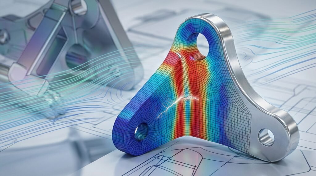
Image courtesy of Wikimedia Commons, depicting stress concentration in a plate.

Understanding Fatigue: The Silent Killer

What is Fatigue?

Fatigue is a progressive, localized structural damage process that occurs when a material is subjected to cyclic or fluctuating stresses and strains. It leads to the initiation and propagation of cracks, eventually causing fracture after a sufficient number of cycles, even if the peak stresses are well below the material’s ultimate tensile strength or even its yield strength.

Why is Fatigue a Critical Engineering Concern?

Consider components in aerospace (aircraft wings, landing gear), oil & gas (risers, offshore platforms), automotive (engine components, chassis), or biomechanics (prosthetics). These systems are constantly subjected to dynamic, repetitive loads. Fatigue failures in such applications can lead to:

Catastrophic Accidents: Sudden, unexpected failures with severe safety implications.
Costly Downtime: Unscheduled maintenance and replacement of parts.
Reputational Damage: Loss of trust in product reliability.
Increased Operating Costs: Frequent inspections and shorter service intervals.

Accurate fatigue life prediction is therefore not just an analytical exercise; it’s a fundamental aspect of safe, economical, and sustainable engineering design.

The Role of FEA in Fatigue Analysis

Bridging Theory and Practice

Traditionally, fatigue analysis relied heavily on empirical data, S-N curves from testing, and simplified analytical models. While these methods are foundational, they often struggle with complex geometries, intricate loading conditions, and heterogeneous materials. FEA offers a powerful bridge, allowing engineers to:

Accurately determine stress and strain distributions in complex components.
Identify stress concentration points, which are prime locations for crack initiation.
Evaluate the impact of design changes on fatigue performance early in the design cycle.
Simulate various loading scenarios (e.g., variable amplitude loading) that are difficult or expensive to test physically.

Advantages of FEA for Fatigue

Using FEA for fatigue life prediction brings several advantages:

Detailed Stress Insight: Visualizing stress and strain fields, especially at geometric discontinuities.
Parametric Studies: Easily modifying design parameters (e.g., fillet radii, hole sizes) to optimize fatigue performance.
Cost-Effectiveness: Reducing the need for extensive physical prototyping and testing, particularly for expensive components or large structures.
Faster Iteration: Accelerating the design-analysis-refine cycle.
Complex Loading: Handling non-proportional loading, multi-axial stress states, and load histories.

Essential Concepts for FEA-Based Fatigue Life Prediction

Before diving into the FEA workflow, it’s crucial to grasp the core concepts.

Stress-Life (S-N) Approach

The S-N approach, also known as the high-cycle fatigue (HCF) approach, is based on experimental curves (S-N curves) that plot stress amplitude (S) against the number of cycles to failure (N). It’s primarily used when stresses are elastic or primarily elastic, and component life is typically greater than 10⁴ cycles.

Key Input: Stress amplitude, mean stress, material S-N curve.
Output: Number of cycles to failure.
Limitations: Does not explicitly account for plastic deformation; sensitivity to surface finish, residual stresses.

Strain-Life (ε-N) Approach

The ε-N approach, or low-cycle fatigue (LCF) approach, is more suitable when significant plastic deformation occurs (e.g., at stress concentrations) and component life is typically less than 10⁴-10⁵ cycles. It uses strain amplitude versus cycles to failure curves.

Key Input: Strain amplitude, material ε-N curve, cyclic stress-strain curve.
Output: Number of cycles to failure.
Advantages: Better accounts for localized plasticity and is more accurate for LCF regimes.

Key Parameters: Stress Concentration, Mean Stress, Surface Finish

Stress Concentration: Geometric discontinuities (holes, fillets, notches) cause local stress amplification, which significantly reduces fatigue life. FEA excels at identifying these hotspots.
Mean Stress: The average stress in a load cycle. A tensile mean stress generally reduces fatigue life, while a compressive mean stress can extend it. Various mean stress correction theories (e.g., Goodman, Soderberg, Gerber, Smith-Watson-Topper) are applied.
Surface Finish: Surface roughness, residual stresses from manufacturing (machining, shot peening), and surface treatments greatly influence fatigue crack initiation.

Material Properties: What You Need

Accurate material data is the bedrock of reliable fatigue analysis. For FEA, you’ll need:

Elastic Properties: Young’s Modulus, Poisson’s Ratio.
Tensile Properties: Yield Strength, Ultimate Tensile Strength.
Fatigue Properties:
- For S-N: Fatigue strength coefficient (σ’_f), fatigue strength exponent (b), fatigue ductility coefficient (ε’_f), fatigue ductility exponent (c). Sometimes an endurance limit (S_e) is also considered.
- For ε-N: Cyclic stress-strain curve (if applicable), along with the fatigue ductility and strength parameters.

These properties are typically obtained from extensive material testing.

Practical Workflow for Fatigue Life Prediction using FEA

Here’s a generalized step-by-step workflow. Specific software like Abaqus, ANSYS Mechanical, or specialized fatigue codes (e.g., nCode DesignLife) will have their own interfaces, but the underlying principles remain consistent.

Step-by-Step Guide

Step 1: Geometry & Meshing

CAD Import: Import your 3D CAD model into the FEA pre-processor. Simplify features that don’t significantly affect stress distribution for computational efficiency, but retain all critical features where fatigue is a concern.
Element Types: Use appropriate element types. For 3D solids, tetrahedral or hexahedral elements are common. Consider using parabolic (second-order) elements for better stress accuracy, especially at stress concentrations.
Mesh Density: Crucially, refine the mesh in areas of expected high stress concentration (e.g., fillets, holes, sharp corners). A coarse mesh in these regions will lead to inaccurate stress predictions and unreliable fatigue results.

Step 2: Material Model Definition

Elastic Properties: Define Young’s Modulus and Poisson’s Ratio.
Plasticity (if LCF): If using the ε-N approach or if localized plastic deformation is expected, define the cyclic stress-strain curve or kinematic hardening properties.

Step 3: Load & Boundary Conditions

Cyclic Loads: Apply the fluctuating loads that the component will experience in service. Define the load amplitude, mean load, and frequency.
Boundary Conditions (BCs): Accurately constrain the model to represent how the component is supported in reality. Ensure BCs do not artificially introduce stress concentrations or rigid-body motion.
R-Ratio: Define the stress ratio, R = σ_min / σ_max. This is critical for mean stress corrections.

Step 4: Static/Transient Stress Analysis

Perform a static structural analysis (or transient if loading is dynamic and inertia effects are important) to determine the stress and strain distributions under the peak and trough loading conditions.
Extract stress tensors, stress invariants (e.g., von Mises stress), and principal stresses.

Step 5: Fatigue Solver Application

Integrate the results from the stress analysis with a fatigue solver (either built-in to FEA software like Abaqus/ANSYS or a specialized tool like nCode DesignLife).
Input the material’s S-N or ε-N curves.
Apply mean stress correction theories as appropriate.
Define the load history if it’s not constant amplitude.

Step 6: Post-Processing & Interpretation

Life Contour Plots: Visualize the predicted fatigue life distribution across the component. Identify critical locations with the shortest life.
Damage Accumulation: For variable amplitude loading, use damage accumulation rules (e.g., Miner’s Rule) to sum damage from different load blocks.
Safety Factors: Evaluate safety factors against target life.

For more advanced post-processing or integration with other tools, you might find Python scripting for Abaqus or similar automation particularly useful for extracting and manipulating large datasets.

Choosing the Right Fatigue Method

Selecting between S-N and ε-N depends on the loading and material response:

Feature	Stress-Life (S-N) Approach	Strain-Life (ε-N) Approach
Loading Regime	High-Cycle Fatigue (HCF)	Low-Cycle Fatigue (LCF)
Stress/Strain Level	Primarily elastic stress	Significant plastic strain
Typical Life (Cycles)	> 10⁴ to 10⁷+	< 10⁵
Material Behavior	Elastic	Elastic-plastic
Crack Focus	Crack initiation (surface)	Crack initiation (sub-surface) & early propagation
Input Data	S-N curve, UTS, Yield Strength	ε-N curve, Cyclic Stress-Strain curve
Software Suitability	Good for general design (Abaqus, ANSYS)	Better for localized plasticity (Abaqus, ANSYS with advanced material models, nCode)

Leveraging Tools: Abaqus, ANSYS Mechanical, nCode DesignLife

Abaqus: Offers robust capabilities for both static and cyclic analysis, including advanced material models for plasticity and built-in fatigue evaluation tools (e.g., fe-safe integration).
ANSYS Mechanical: Provides comprehensive tools for structural analysis and integrates with fatigue modules like ANSYS nCode DesignLife or its native fatigue tools to perform life predictions using various methods.
nCode DesignLife: A specialized fatigue analysis software that integrates with FEA results from various solvers (Abaqus, ANSYS, Nastran, etc.). It’s highly regarded for its extensive material database, multiaxial fatigue capabilities, and ability to handle complex load histories.

Verification & Sanity Checks for Robust Fatigue Analysis

Garbage in, garbage out. A critical part of any FEA is verifying the results. For fatigue analysis, this is even more crucial due to the sensitivity of life predictions to input parameters.

Mesh Sensitivity Studies

Perform analyses with progressively finer meshes, especially in critical regions. The results (e.g., peak stress, predicted life) should converge to a stable value. If they don’t, your mesh is likely too coarse in those areas.

Boundary Condition Validation

Ensure your applied loads and boundary conditions accurately represent the real-world scenario. A simple hand calculation or analytical model can often serve as a sanity check for reaction forces or global displacements.

Material Data Accuracy

The material’s fatigue properties (S-N/ε-N curves) are highly sensitive. Confirm the source of your material data. Generic data may not be sufficient; specific tests on the actual material lot might be necessary for critical applications.

Analytical/Hand Calculation Cross-Checks

For simplified regions or components, compare FEA results against classical fatigue formulas (e.g., using Neuber’s rule for stress concentration or simplified endurance limit calculations). This provides a quick reality check.

Convergence Criteria for Stress Results

In non-linear analyses (common for ε-N approach), ensure solution convergence is achieved. Check for error norms and energy balance. Divergent or poorly converged solutions will yield meaningless fatigue lives.

Sensitivity to Input Parameters

Conduct a sensitivity study on key input parameters such as load magnitude, material properties, and mean stress corrections. Understand how variations in these parameters affect the predicted fatigue life. This is particularly important for fracture critical components or FFS Level 3 assessments.

Common Pitfalls and How to Avoid Them

Even experienced engineers can fall into these traps:

Ignoring Mean Stress Effects

Assuming constant amplitude fatigue with zero mean stress can lead to dangerously optimistic life predictions if a significant mean stress exists. Always consider mean stress correction theories.

Inadequate Meshing at Hotspots

This is arguably the most common error. A coarse mesh will smooth out stress gradients, underpredicting peak stresses and overpredicting fatigue life. Always refine the mesh at stress concentration points.

Using Generic Material Data

Material properties, especially fatigue ones, vary significantly with manufacturing process, heat treatment, and even batch. Relying on textbook values for critical designs is risky. Seek specific material test data.

Overlooking Residual Stresses

Manufacturing processes (welding, machining, shot peening) can induce significant residual stresses. Compressive residual stresses can be beneficial, while tensile ones can be detrimental to fatigue life. These often need to be included in the FEA if significant.

Misinterpreting Results

Fatigue life prediction is probabilistic. A predicted life of ‘X’ cycles doesn’t mean it will fail exactly at ‘X’. It’s a statistical estimate. Understand the scatter in fatigue data and use appropriate safety factors. Also, remember that FEA typically predicts crack initiation life, not total life (which includes crack propagation).

Enhancing Your Fatigue Analysis Skills

Mastering fatigue life prediction with FEA requires continuous learning and practice. EngineeringDownloads.com offers resources to help you deepen your understanding and refine your skills. Explore our collection of downloadable example project files for Abaqus or ANSYS, practical Python scripts for automating CAE post-processing, or consider specialized online tutoring for advanced topics like Fitness-for-Service (FFS) Level 3 assessments and damage tolerance analysis.