Introduction

Fatigue failure is one of the most common causes of unexpected breakdowns in engineering structures subjected to cyclic loading. Even when stresses are well below a material’s yield or ultimate strength, repeated load cycles can initiate small cracks that grow over time, eventually leading to catastrophic fracture. Predicting fatigue life (the number of cycles to failure) is therefore crucial in industries like oil & gas (pressure vessels, pipelines), aerospace (aircraft wings, engine components), automotive (suspensions, crankshafts), and civil engineering (bridges, offshore structures). Modern Finite Element Analysis (FEA) tools such as ANSYS and Abaqus play a key role in fatigue assessments by calculating detailed stress/strain distributions in complex geometries. By combining FEA results with fatigue material data and design codes (e.g., ASME boiler & pressure vessel standards, API 579-1/ASME FFS-1 Fitness-For-Service guidelines), engineers can estimate how long a component will last under cyclic loads and how to improve its durability. In this comprehensive guide, we’ll cover the fundamentals of fatigue, the difference between crack initiation and crack propagation, and how various FEA-based tools (ANSYS, Abaqus, fe-safe, MSC Fatigue, FEMFAT, Zencrack, etc.) are used in fatigue analysis and life prediction. The tone is friendly and accessible – as if we’re walking through the topic together – but with the depth needed to make this the go-to resource on fatigue in FEA.

What is Fatigue and Why Does it Matter?

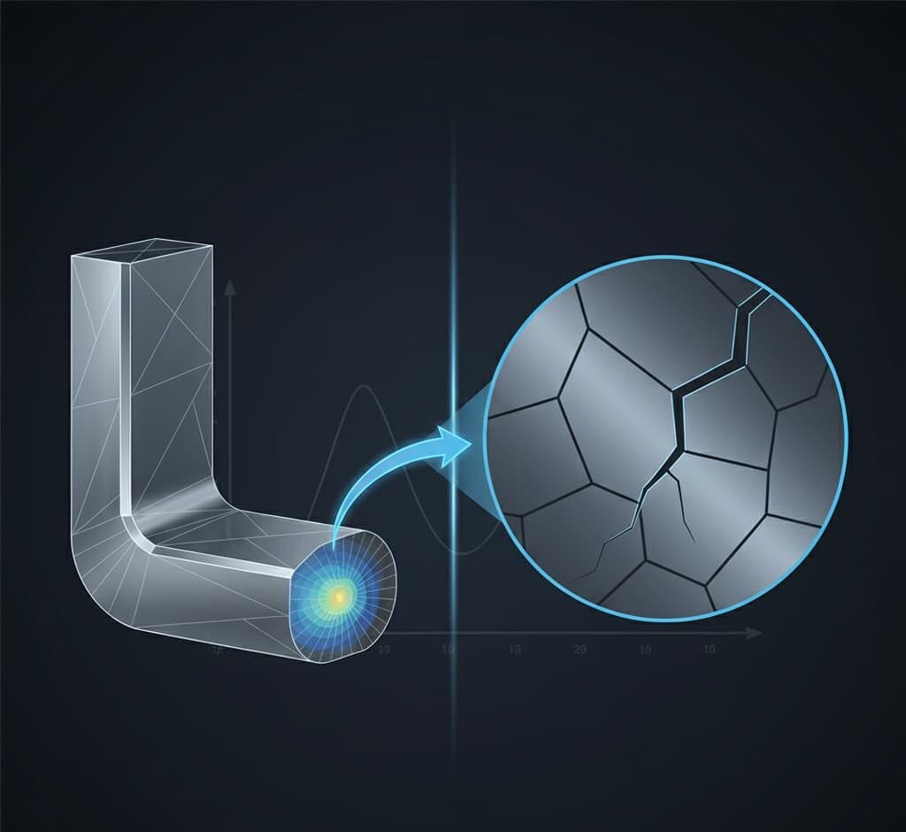
Fatigue refers to the progressive, cumulative damage that materials endure under repeated fluctuating stresses. Unlike an overload failure which happens instantly when a load exceeds strength, fatigue failure happens over time: each load cycle causes a tiny amount of damage. Initially, micro-cracks form at points of high stress (for example, around a scratch, weld toe, or pore in the material). With each subsequent cycle, these cracks initiate and propagate further, until the remaining cross-section of the part is too weak to carry the load, resulting in sudden fracture without warning. In fact, a component can fail from fatigue at stress levels much lower than its static strength because the damage accumulates over millions of cycles. This makes fatigue especially insidious and important to predict – failures in service can be costly or dangerous (think of a bridge collapsing after years of traffic, or an oil rig pipeline leaking due to cyclic pressure swings).

Fatigue life generally consists of two stages: crack initiation and crack propagation. In the initiation phase, tiny cracks nucleate at material defects or stress concentrators (like sharp corners, weld defects, surface roughness). This could consume a significant portion of the life for ductile, high-quality materials – the material endures many cycles of micro-damage before a crack is visible. Once a crack has formed, the propagation phase begins where the crack gradually grows in length with each cycle. Eventually, the crack reaches a critical size at which the remaining material can no longer support the load, and final fast fracture occurs. Both stages are important: some designs aim to prevent crack initiation entirely over the expected life, while others allow a crack to form but use periodic inspections and fracture mechanics to ensure the crack will not grow to failure before detection and repair. In designing against fatigue, engineers must consider things like the stress levels, how often and in what manner loads are applied, material properties (including any treatments like surface hardening), and the environment (corrosion can accelerate fatigue). Check out our Crack Propagation package for more examples:

High-Cycle vs Low-Cycle Fatigue

Not all fatigue is equal – the nature of the loading (high vs low amplitude, many vs few cycles) affects the failure mechanism and how we predict it. High-Cycle Fatigue (HCF) typically refers to situations where the number of cycles to failure is very large (in the order of 10,000 to millions of cycles) and the stress levels are relatively low, largely in the elastic range of the material. Because deformations remain elastic, each individual cycle causes only a tiny damage, but the huge number of cycles can still result in failure. High-cycle fatigue is common in things like vibrating machinery, rotating shafts or turbine blades, where loads are frequent but not causing visible yielding. Low-Cycle Fatigue (LCF), on the other hand, involves higher stress amplitudes often causing plastic deformation, and failure occurs in a relatively low number of cycles (perhaps <10,000 cycles). LCF is typically associated with scenarios like startup/shutdown thermal strains in equipment, seismic loads, or anything that plastically strains the material each cycle – the material can endure fewer such cycles because each one does significant damage.

In design and analysis, HCF is usually handled with a stress-life (S–N) approach (described below) because we assume elastic behavior and long life, whereas LCF often demands a strain-life (ε–N) approach because we must account for plastic strain energy per cycle. An interesting middle ground is Thermo-Mechanical Fatigue (TMF) – where cyclic thermal stresses (due to temperature changes) combine with mechanical loads – but that’s beyond the basics here. The key takeaway is that whether you expect 100 cycles or 10 million cycles changes how you assess fatigue. (Often, the cutoff between LCF and HCF is not a sharp line but engineers use ~10⁴ or 10⁵ cycles as a rule-of-thumb boundary.)

Cyclic Loading Patterns and Mean Stress Effects

Not only the magnitude and count of cycles matter – the pattern of cyclic loading also influences fatigue damage. Consider the difference between a fully reversed load versus a fluctuating load with a nonzero mean. A fully reversed cycle (like alternating tension and compression of equal magnitude, e.g. stress goes from +X to –X) has a stress ratio R = –1 (ratio of minimum to maximum stress). Many laboratory fatigue tests use this kind of loading to generate material S–N curves under zero mean stress. In real-world conditions, however, loads often fluctuate between a maximum and a minimum that are both positive (e.g. 0 to X, or Y to X with Y > 0). This introduces a mean stress component – a positive mean stress (tension bias) tends to reduce fatigue life, because the material has less “breathing room” for crack faces and is under tension even at the minimum of the cycle. Conversely, a compressive mean can extend life (though materials rarely fail under full compression fatigue). Engineers use mean stress correction methods to account for this when using material data. Two common visualization tools are the Goodman and Haigh diagrams, which plot mean stress vs alternating stress to delineate safe and failure regions.

Mean stress correction illustrated on a fatigue limit diagram. The Gerber parabola (curved line) and the linear Goodman line both approximate the combination of mean and alternating stress that leads to failure. The Soderberg line (most conservative) uses yield strength as a limit.

Goodman’s line is a linear relation that connects the material’s endurance limit (at zero mean stress) to its ultimate tensile strength (at which zero alternating stress can be endured). It provides a conservative estimate of allowable stress amplitude for a given mean stress. Gerber’s parabola is a curved relation that fits experimental data more closely for ductile metals – it is less conservative than Goodman (except at the extremes) and often used when a better fit is needed. Soderberg’s line connects the endurance limit to the yield strength, and is very conservative (often unduly so, rarely used unless a high safety factor is needed). In practice, if you have an S–N curve for zero mean stress (fully reversed, R = –1 conditions), you can use these relations to adjust for a different mean. Modern fatigue analysis software (including ANSYS Mechanical’s fatigue tool) often lets you choose a mean stress correction: Goodman, Soderberg, Gerber for stress-life analysis, or other models for strain-life (like Morrow or Smith-Watson-Topper (SWT) which account for mean strains/stresses in low-cycle fatigue). The general trend, of course, is that increasing tensile mean stress shortens fatigue life – so designs that can reduce mean stress (e.g. by stress relieving, prestressing, or using symmetric loading) will improve fatigue performance.

Another aspect of loading is whether cycles are constant amplitude or variable amplitude. Many structures experience a spectrum of different load levels. For example, a truck frame sees occasional heavy loads and many lighter bumps – not all cycles are equal. Fatigue damage from variable loading is typically assessed by breaking the history into equivalent cycles using methods like rainflow counting (per ASTM E1049), then applying a cumulative damage rule (most commonly Miner’s Rule which sums damage fraction linearly). Essentially, each distinct range of stress contributes a fraction damage = cycles_applied / cycles_to_fail at that range, and if the sum of damage fractions ∑D reaches 1.0, fatigue failure is expected. This linear damage rule is a simplification (it neglects sequence effects, etc.), but it’s widely used in industry and supported in fatigue analysis tools.

Approaches to Fatigue Life Prediction

Predicting fatigue life can be approached from a few different angles, depending on the available data and the nature of the problem. The three primary methods are the stress-life approach, strain-life approach, and fracture mechanics approach:

• Stress-Life (S–N Curve) Approach: This is the traditional method, also called the Wöhler curve approach. It is based on empirical S–N curves that relate stress amplitude to the number of cycles to failure on a log-log plot. Engineers conduct fatigue tests at various stress levels and record the cycles to failure to establish the curve. Using this method, if you know the stress range (often the alternating stress \sigma_a) in your component, you can directly read or interpolate the number of cycles to failure (N_f) from the S–N curve. The stress-life method works well for high-cycle fatigue where deformations are elastic. It’s convenient because many design codes (like ASME VIII-2 for pressure vessels) provide S–N curves for different materials that already include surface finish factors, etc. However, it doesn’t explicitly separate crack initiation from growth – it just gives total life. Also, the S–N method struggles with situations involving significant plasticity or nonzero mean stress (which we address via correction factors as discussed above). Still, for things like a steel shaft under alternating bending, an S–N approach (with a Goodman correction if needed) is often the quickest way to estimate fatigue life.
• Strain-Life (ε–N Curve) Approach: When loads are severe enough to cause plastic deformation each cycle (low-cycle fatigue), the strain-life approach is more appropriate. Instead of stress amplitude, it uses strain amplitude (often split into elastic and plastic components) versus cycles to failure. A well-known formulation is the Coffin-Manson relation for low-cycle fatigue, which, in combination with the Basquin relation for elastic cycles, leads to the total strain-life equation:

\frac{\Delta \varepsilon}{2} = \underbrace{\frac{\sigma_f'}{E\,(2N_f)^b}}_{\text{elastic strain}} + \underbrace{\varepsilon_f'(2N_f)^c}_{\text{plastic strain}}

Here 2N_f is reversals to failure (twice cycles), \sigma_f', b, \varepsilon_f', c are fatigue strength and ductility coefficients and exponents respectively (material properties obtained from tests). Don’t worry if that looks complex – the key point is the strain-life method accounts for both elastic and plastic strain energy. It effectively captures LCF behavior, where a component might fail after, say, 500 plastically ratcheting cycles. Modern fatigue software will let you input these ε–N parameters or derive them from material tensile properties. The strain-life method also can incorporate mean stress effects (e.g., using Morrow’s correction which subtracts mean stress from the endurance term, or SWT which uses the product of max stress and strain amplitude). Use strain-life when your component sees yielding – for example, thermal expansion in a constrained tube that yields each heat-up/cool-down cycle.

• Fracture Mechanics (Crack Growth) Approach: The two methods above are largely crack initiation methods – they predict the total life to failure without explicitly modeling a crack. In contrast, the fracture mechanics approach assumes a crack (or flaw) is present (or will inevitably form) and focuses on predicting crack propagation life. This approach is crucial for damage tolerance and fitness-for-service (FFS) evaluations: rather than asking “How many cycles till this part breaks from new?”, we ask “If there is a crack of size a_0, how many cycles until it grows to an unsafe size a_{\text{crit}}?”. The crack growth rate per cycle, da/dN, is typically modeled by the Paris-Erdogan law (for the mid-range of crack growth behavior):
  \frac{da}{dN} = C \left( \Delta K \right)^{m}
  where ΔK is the stress intensity factor range for the crack (a function of stress, crack size, and geometry), and C and m are material constants obtained from lab tests. Paris law basically says crack growth per cycle is a power-law function of how “intense” the stress field at the crack tip is (ΔK). There are more elaborate models (to handle threshold effects at low ΔK, or fast fracture as K→K_c, but Paris law is the workhorse for fatigue crack growth calculations. Using it, engineers can integrate da/dN over cycles to predict how a crack grows from a_0 to a_{\text{crit}}. Fracture mechanics is especially useful for components that already have flaws (welded structures with initial cracks, or an inspected part with a known defect). In fact, standards like API 579-1/ASME FFS-1 include procedures for crack growth analysis: e.g. given an initial flaw size from inspection, you can calculate remaining life before it reaches critical size. Fitness-for-Service assessments often combine this with inspection intervals – ensuring that cracks won’t grow to failure before the next planned inspection.

It’s worth noting that in many design scenarios, engineers use a combination: an S–N approach to ensure no fatigue failure in the initiation phase for a certain life, and a fracture mechanics approach to ensure that if a crack does form (perhaps after that design life or due to some anomaly), it will grow slowly enough to be detected and repaired. For example, DNV-RP-C203 (a recommended practice for offshore structures) explicitly separates fatigue design into initiation and propagation phases, with methods to address each. In safe-life designs (like many aircraft parts), the aim is to keep total life (initiation+propagation) beyond the service life with a safety factor. In damage-tolerant designs, the aim is to manage propagation via inspections.

Using Finite Element Analysis in Fatigue

So, how do finite element simulations come into play for fatigue? FEA is an invaluable tool to predict stress and strain distributions in components under complex loads. Since fatigue life depends heavily on the local cyclic stress/strain at critical spots, FEA helps identify those “hot spots” and provides the stress ranges needed for life calculation. The typical workflow is: use an FEA solver (like ANSYS, Abaqus, Nastran, etc.) to model the component and apply the cyclic loads (or representative static loads that produce the stress extremes). The FEA results will give you stress (or strain) at each point in the structure. Then, use a fatigue post-processing tool or calculation to estimate life at those points. Essentially, FEA provides the input (stress range, mean stress) for the fatigue models we discussed earlier (S–N or ε–N curves, etc.).

For example, if analyzing a welded pressure vessel nozzle under pressure cycles: an FEA might show that the highest stress range is at the weld toe. Taking that stress range, you consult an S–N curve for welded joints (perhaps from ASME or IIW standards) and find the fatigue life. If multiple load cases or a spectrum, you might use FEA to get stress responses for each case and then do a cumulative damage calculation. FEA is particularly powerful for complex geometries where stress concentrations are not obvious or where stress varies spatially. It allows fatigue “hot spot” analysis: plotting a contour of fatigue life over the model to see where failure would likely initiate first.

It’s important to note that standard FEA (elastic stress analysis) itself does not directly give fatigue life – it provides stresses. The fatigue life prediction is a subsequent calculation. Some FEA software do have built-in fatigue modules or allow certain direct fatigue simulations (we’ll discuss these in the tool-specific section). One interesting capability in Abaqus is the “direct cyclic analysis”, which can find the stabilized response of a structure under repeated loading without simulating every cycle – useful for analyzing shakedown and ratchetting. However, even direct cyclic analysis by itself stops short of giving “cycles to failure”; it might be used in conjunction with a continuum damage model or to compute things like energy dissipation per cycle which correlate to life. Similarly, one can implement continuum damage mechanics (CDM) in FEA – essentially, degrade the material stiffness a bit each cycle based on a damage variable until failure – but this often requires a user subroutine or special material model (and good calibration). For most practical purposes, engineers rely on FEA for stresses and specialized fatigue codes for life.

The accuracy of fatigue predictions via FEA depends on a few factors: quality of the stress analysis (mesh refinement at stress concentrators, correct representation of loads and boundary conditions), quality of the material fatigue data (S–N curve, etc., relevant to the actual surface finish and environment of the part), and accounting for any mean stress or multi-axial effects. Multi-axial fatigue (non-proportional loading where principal stress directions change) is a whole topic on its own – advanced fatigue software use critical plane searching algorithms to find the orientation that maximizes damage. If you suspect multi-axial stresses (like a shaft with combined bending and torsion), it’s best to use a tool that can handle that (or convert to an equivalent uniaxial stress via von Mises or some criterion, with caution).

Finally, FEA helps in design iteration for fatigue: you can modify geometry (add a fillet, remove a notch) and recompute stresses to see if the fatigue hot spot stress is reduced, thereby improving life. You can also evaluate the effect of residual stresses (for example from welding or shot-peening) by including them in the FEA – compressive residual stress at the surface often improves fatigue life significantly, and some fatigue tools allow you to input a residual stress field or a mean stress offset.

In summary, FEA is the microscope that reveals where and how the part is stressed; the fatigue calculations then predict how long those stressed areas will last under repeated loading. Now, let’s look at specific software tools and how they facilitate fatigue analysis.

Fatigue Analysis Tools in FEA Software

Fatigue analysis can be performed with a combination of general FEA solvers and specialized fatigue post-processing programs. Here we discuss some popular tools and how they approach fatigue:

ANSYS Mechanical – Integrated Fatigue Module

ANSYS Mechanical (Workbench) has a built-in fatigue module that allows users to perform fatigue life calculations directly after a stress analysis. Once you have run a static or transient FE analysis to get the stress results, you can insert a Fatigue Tool in ANSYS Workbench and define the fatigue parameters. ANSYS supports both stress-life (SN) and strain-life (EN) approaches. You can input an S–N curve for the material (or multiple curves at different R ratios). For strain-life, you input Coffin-Manson parameters. The software can handle constant amplitude fatigue easily and also does rainflow counting for variable amplitude load histories. A nice feature is it outputs fatigue life contours on your model, so you can see the predicted life at every point (or a safety factor for a given life).

ANSYS’s fatigue tool also includes options for mean stress corrections – as discussed, you can select None, Goodman, Gerber, or Soderberg for stress-life calculations. If you have multiple S–N curves at different mean stresses, you can even have it interpolate (“Mean Stress Curves” option). For strain-life, ANSYS offers mean stress models like Morrow and SWT, which adjust the damage calculation for nonzero mean strains. This helps improve accuracy when your FEA stress had a bias (say you did a pre-load plus alternating load). ANSYS can also account for multiaxial stress states to some extent – for proportional loading it might use an equivalent stress amplitude (like von Mises or signed von Mises), but for nonproportional fatigue a more advanced critical plane approach is needed (ANSYS natively doesn’t do a full critical plane search in the basic module, but it can interface with other tools for that).

For crack propagation analysis, ANSYS doesn’t have an out-of-the-box automated crack growth tool in Workbench; however, ANSYS can be used with custom scripts or with external crack growth software. ANSYS Mechanical APDL does have some fracture mechanics calculation capabilities (like stress intensity factor computation via contour integrals, etc., and there is a separate tool called ANSYS Virtual Crack Growth for simple crack cases). But generally, for fatigue crack growth, one would export results to a tool like NASGRO or use an add-on.

It’s worth noting that ANSYS has partnerships with other fatigue software too. For instance, nCode DesignLife (by HBM, now part of Altair) is a widely used fatigue post-processor that can take ANSYS results. Some ANSYS packages actually bundle an nCode license. DesignLife can do more advanced analyses (like spot weld fatigue, vibration fatigue, etc.), but if you have ANSYS Workbench, the built-in fatigue module is often sufficient for standard tasks. Overall, ANSYS provides a fairly seamless experience: you perform an FE analysis and directly get fatigue life or damage as another result type, making life prediction an integrated part of the simulation workflow.

Abaqus & fe-safe – The SIMULIA Solution

Dassault Systèmes’ Abaqus does not have a standalone fatigue life module inside Abaqus/CAE itself for general SN or EN life computations. Instead, the strategy with the SIMULIA suite is to use fe-safe, a dedicated fatigue analysis program that is tightly integrated with Abaqus (and other FEA tools). fe-safe is one of the leading fatigue software packages on the market – it was among the first to focus on modern multiaxial fatigue methods and works directly with FEA results. The typical workflow is: you run an Abaqus analysis (usually a stress analysis under the peak loads or a series of subcases that represent the load cycle turning points), then export the results (like an Abaqus .odb file or results in a universal file format). fe-safe reads those results, along with material fatigue properties you provide, and computes life or damage. It will output contour plots of fatigue life just like an FEA contour – often overlaid on your model – showing where cracks are likely to initiate first.

fe-safe is very powerful: it handles multiaxial fatigue (using critical plane methods to evaluate equivalent damage from complex stress states), non-zero mean stresses, welded joints (it has the Verity module which is a special algorithm for weld fatigue using structural stress method), and even elastomer fatigue (fe-safe/Rubber module for things like rubber mounts, which use different failure criteria). It supports both stress-life and strain-life, includes a material database, and can do cumulative damage for load histories (including random vibration fatigue in frequency domain!). Essentially, fe-safe takes the grunt work of looping through every node’s stress history and calculating fatigue damage – something not practical to do manually on large models – and does it efficiently. It directly interfaces with all major solvers (Abaqus, ANSYS, MSC Nastran, etc.).

For Abaqus users, fe-safe is the go-to solution for fatigue initiation life predictions. If you are using Abaqus and need to predict when/where cracks might form under cyclic loads, you’d use fe-safe. Abaqus itself can simulate some damage evolution via user subroutines (for example, a UMAT that gradually degrades material as a function of cycles), but that requires significant expertise. There is also an Abaqus add-on called Abaqus fatigue module, but it’s basically a plugin that still uses fe-safe in the background or simplified methodology for certain cases. In recent versions, Abaqus has introduced some features for low-cycle fatigue in the material models (like the ability to define a cyclic damage initiation criterion and progressive damage for metals), which can be used to simulate crack initiation directly in Abaqus (for example, using XFEM to allow a crack to initiate and grow when a certain damage parameter reaches a threshold). One example is simulating a crack propagating via the extended finite element method (XFEM) using a criterion based on Paris law – indeed, Abaqus allows specifying a Paris-law-based growth rate in a direct cyclic analysis step for crack growth, and some have used the direct cyclic technique with XFEM to simulate a crack growing incrementally each cycle (without remeshing). However, these approaches are advanced and typically used in research or special cases. For most engineering purposes, one would do an Abaqus stress analysis and then use fe-safe for life prediction (initiation). Check out our example in Fatigue Life Estimation using Abaqus and Fe-Safe!

MSC Fatigue (MSC Nastran/Marc add-on)

MSC Fatigue is a fatigue life estimation package from MSC Software (now part of Hexagon). It works similarly to fe-safe in that it uses FEA results from MSC Nastran, Patran, Marc or others, and computes fatigue life. MSC Fatigue has been around for quite a long time as well – it was known for a broad range of fatigue capabilities: from simple stress-life to strain-life, spot weld and seam weld fatigue, vibration fatigue, etc. It’s often used in aerospace and automotive sectors that historically used MSC Nastran for stress analysis. For example, an engineer might run a Nastran analysis on a car chassis, then use MSC Fatigue to predict how many miles of road usage until fatigue cracks might appear in the chassis. MSC Fatigue is integrated with the MSC Patran interface for setting up fatigue analyses, and can also be driven through scripts.

One feature of MSC Fatigue (at least in older versions) was the ability to handle the full spectrum of durability: not just initiation life, but also crack growth to some extent and even fracture (though crack growth might have been handled by a separate tool or module). It’s advertised as the only solution that can deal with the full range of fracture and fatigue, though in practice, specialized crack growth tools are often used for the propagation part. MSC Fatigue includes methods for welded structures (using codes like BS 7608 for weld classification or hotspot stress methods) and can do multi-axial assessments. If you’re using MSC’s structural analysis tools, MSC Fatigue is the natural companion. Its capabilities are on par with fe-safe in many respects (each has its own strengths or ease-of-use differences).

FEMFAT

FEMFAT (short for Finite Element Method Fatigue) is another popular fatigue analysis software, originally developed by Austrian company Magna Steyr. It is widely used in the automotive industry for durability analysis. FEMFAT reads results from most FEA codes and has modules for different types of fatigue: e.g., FEMFAT base (for standard stress/strain-life), FEMFAT weld (for welded structures), FEMFAT spot (for spot welds), FEMFAT brake (for thermomechanical fatigue in brake discs), etc. Automotive companies often use FEMFAT to predict fatigue life of chassis components, engine parts, etc., under proving ground load histories. Like fe-safe and MSC Fatigue, it provides life or damage contours, supports multiaxial criteria (like critical plane methods), and has material libraries. One notable feature of FEMFAT is its focus on spot weld fatigue – it has specialized algorithms to predict fatigue in spot-welded sheet metal structures (important for vehicle bodies). It also can handle frequency domain fatigue analysis which is useful for vibrating components (random vibration loading given by PSDs).

In terms of workflow, if you had an ANSYS or Abaqus or Nastran stress analysis done, you could import the stresses into FEMFAT, define the materials and loading (it can apply multiple load channels and scale them to mimic a duty cycle), and run the fatigue calculation. FEMFAT will then show you which element or node fails first and at how many cycles. Many large companies calibrate FEMFAT predictions with physical test data to refine their parameters for better accuracy.

In summary, fe-safe, MSC Fatigue, and FEMFAT all fulfill a similar role: they take FEA results and compute fatigue crack initiation life at points in the structure. They differ in interface and some advanced capabilities, but an expert can often get comparable results from each if used correctly.

One thing to clarify: these tools (fe-safe, MSC Fatigue, FEMFAT) primarily address the initiation phase of fatigue – i.e., when and where a crack will start. They typically do not simulate the actual crack propagating through the model (that’s a different type of simulation as discussed with fracture mechanics). Instead, they assume failure when a crack initiates to a certain small size (like ~1-2 mm). For many design purposes, that’s fine because a “failed” component is one that has cracked even if it hasn’t broken in two yet. But if you need to simulate what happens after the crack forms, you need crack growth analysis.

Zencrack – Simulating Crack Propagation

For simulating fatigue crack growth (propagation) with FEA, Zencrack is a well-known tool. Zencrack (by Zentech) is essentially an automated crack growth simulation program that works with FEA solvers like Abaqus. It uses fracture mechanics: you start with an initial crack (you actually insert a crack in your FE model, like a crack in a solid or shell, with a specific size and location). Zencrack then performs cycles of analysis where it: calculates stress intensity factors (K) or energy release rate (J-integral) at the crack front from the FEA results, uses a crack growth law (like Paris law) to increment the crack a little bit, automatically updates the FE mesh to extend the crack (remeshing or node release), and repeats for the next increment. In this way, it “grows” the crack step by step through the component, until either a target crack size is reached or the crack causes failure. Zencrack can handle complex 3D cracks and can grow them in arbitrary directions depending on the stress field (it often includes criteria to predict crack turning, etc.). It is particularly useful for things like: “Will a crack at this weld toe grow into the thickness and cause leakage by 100,000 cycles?” or “What is the crack path in a bracket under bending fatigue?”.

Using Zencrack requires some expertise because you have to have a good initial FE model with a crack and understand fracture mechanics inputs (Paris law C, m, etc., and perhaps threshold and fracture toughness). But it’s an extremely powerful approach for damage tolerance analysis – e.g., aerospace industry uses such tools to ensure that even if a crack starts, it will take a certain number of cycles to reach critical so that inspections can catch it. Some regulatory standards require explicit demonstration of crack growth life in safety-critical structures (e.g., aircraft fuselage).

Zencrack is often used in conjunction with Abaqus: Abaqus provides the stress analysis for each crack length configuration. In fact, Zencrack can automatically set up an Abaqus job, read results, and modify the Abaqus input to extend the crack. There are other crack growth tools as well (e.g., FRANC3D, NASGRO for simpler cases, etc.), but Zencrack is notable and was explicitly asked about. The key point is: crack propagation simulation is a different domain from the S–N or ε–N life prediction. It’s more computationally intensive (multiple FEA runs as the crack grows) but gives a very detailed picture of how a crack advances. It’s used when you need that level of detail, usually after a crack has been found or for critical parts where you assume a crack will start at some life.

Industry Codes and Standards in Fatigue Analysis

Fatigue analysis doesn’t happen in a vacuum – industry codes and standards provide guidelines to ensure safety and consistency. When performing fatigue assessment for real projects (especially in regulated industries like pressure vessels, pipelines, aerospace), engineers must align with these standards:

• ASME Boiler & Pressure Vessel Code (BPVC): ASME Section VIII Division 2 (“Design by Analysis” section) includes a detailed fatigue evaluation procedure for pressure vessels. It provides fatigue design curves for various materials (plots of stress amplitude vs cycles for design purposes) and specifies how to calculate a fatigue usage factor. Essentially, an ASME Div.2 fatigue assessment involves determining the stress ranges from a stress analysis (often an FEA of the vessel or component), categorizing them (membrane, bending, etc.), and then counting cycles for each load case. You then use the provided S–N curves (which are typically mean plus two standard deviation curves for conservative life) to find allowable cycles, compute the damage fraction for each, and sum them (Miner’s rule). The vessel is acceptable if the total usage factor ≤ 1 (or ≤ some allowable like 0.5 for design, etc., depending on code). ASME code also gives guidance on factors like surface finish, temperature, size effect which might adjust the allowable stress or life. For welded details, ASME might refer to other standards or provide its own classification of welded joint fatigue strength. The takeaway: if you’re designing a pressure vessel or piping for cyclic service, you’ll likely follow ASME procedures to show adequate fatigue life. Modern FEA makes it easier to get the needed stresses (for example, some software like ANSYS have built-in ASME fatigue tools where you input the ASME curve and it computes usage).
• API 579-1 / ASME FFS-1 (Fitness-For-Service): This is a recommended practice used mostly in the oil & gas and petrochemical industry for evaluating existing equipment that may have flaws or damage. Part 14 of API 579-1 (added in the 2016 edition) is specifically about Fatigue Assessment. It provides guidelines for evaluating remaining life due to fatigue for equipment that’s already in service. For example, if an in-service pressure vessel experienced more cycles than originally anticipated, or if inspections show some cracking, Part 14 gives methods (Level 1, 2, 3 assessments of increasing complexity) to estimate remaining life. A Level 1 might be a conservative screening using design curves, Level 2 might allow some measured data usage, and Level 3 could involve detailed FEA and crack growth analysis. The standard also has guidance on welded joint categories and how to adjust life for welds (since welds often are the most fatigue-sensitive locations). The fitness-for-service (FFS) approach is often about being conservative yet avoiding unnecessary scrap of equipment – you demonstrate that even with existing flaws, the equipment can run safely for X more cycles. API 579’s fatigue methods complement the ASME design-by-analysis: ASME might have been used to design initially, and API 579 is used later to assess if it’s still okay when actual loads and conditions are known. If you are doing a consultancy project for an aging refinery unit that has cyclic temperature swings, you might perform an FEA of the component, use the stress results in an API 579 fatigue calculation to see if it will last another 5 years, or if not, what mitigation is needed.
• Industry-specific standards: As mentioned earlier, DNV-RP-C203 is used in offshore structures (oil rigs, etc.) to ensure fatigue life of welds and structural nodes under wave loading. IIW guidelines for welds are used widely for welded steel structures – they provide categories of welded details and associated S–N curves (for example, a transverse non-load-carrying attachment weld might be Category 80 with a certain curve slope). Eurocode for bridges, AASHTO for bridge fatigue, MIL-STD-1530 etc. for aircraft fatigue, and so on – each industry has its rules. In automotive, durability targets are often based on road load spectra and company-specific tests, but standards like SAE papers provide guidance on how to do accelerated life testing for fatigue. The good news is that all these standards ultimately rely on the same fundamental approaches we’ve discussed: they either give you S–N curves or crack growth rate parameters, and rules on how to apply them.
• Welded Structures: Welds deserve special mention because they typically have much lower fatigue strength than base metal due to residual stress and geometry. Many codes (like AWS D1.1, BS 7608, Eurocode 3, etc.) provide detail categories – basically an S–N curve selection – for different weld types. If your FEA finds a certain stress range at a weld toe, you might not use the base metal S–N curve; you’d use the weld curve which might predict fewer cycles. There are also approaches like the structural stress method or hot-spot stress method where instead of relying on a single element’s stress (which can be mesh-dependent at a weld), you extrapolate surface stress to a hypothetical hot-spot to use in an S–N curve. Tools like fe-safe’s Verity module or FEMFAT weld implement those advanced weld fatigue analysis techniques.

In practice, if you engage in a fatigue analysis project, part of the job is identifying which standard applies and ensuring your analysis is compliant. For instance, if you are doing a fatigue analysis of an offshore crane, you might follow API 2L or DNV guidelines. If it’s a pressure vessel, ASME VIII-2. For a pipeline under cyclic pressure, perhaps API 579 or API 1176. Codes often require conservative assumptions – e.g., assume a surface finish or a certain weld quality. They may also require certain safety factors on life or stress (for example, design fatigue life might need to be 2x the intended life).

Conclusion and Further Support

Fatigue assessment is a blend of engineering science and practical experience. We use theoretical models (S–N curves, crack growth laws, etc.) and real testing data, applied via computational tools like FEA, to predict something that hasn’t happened yet – a crack that might form in the future. While modern software and standards make this easier than ever, it still requires sound judgment: choosing the right method for the situation, interpreting FEA results correctly, and applying appropriate safety factors. A comprehensive fatigue analysis often examines both crack initiation and crack propagation aspects to ensure there are no surprises.

In summary, FEA-based fatigue analysis allows engineers to virtually test their designs for durability. By leveraging tools like ANSYS and Abaqus (with fatigue modules or add-ons like fe-safe, MSC Fatigue, FEMFAT) one can identify weak links in a design and improve them before any physical prototype fails. Meanwhile, using fracture mechanics tools (e.g., Zencrack) provides insight into how cracks grow, which is invaluable for maintenance planning and life extension of existing equipment. And by adhering to ASME, API, and other codes, we ensure that our analysis meets the industry’s reliability and safety benchmarks.

Fatigue can be a complex topic, but it’s also fascinating – it’s where tiny microscale material behaviors meet the macroscale world of bridges, planes, and pipelines. A friendly word of advice: always err on the side of caution with fatigue. If predictions are uncertain, build in extra safety or monitoring. Unlike a static overload, fatigue failures give no warning when they finally let go.

Need help with a fatigue analysis project or want to learn more? Our team at Engineering Downloads offers expert consulting and a specialized fatigue training course (based on ASME & API standards) tailored for the oil and gas industry and beyond. We can help with everything from setting up FEA models for fatigue, to interpreting results, to applying code criteria, and even train your engineers in these techniques. Feel free to reach out for professional assistance or check out our resources and courses on our website. We’re passionate about helping engineers solve their toughest fatigue problems – and ensuring your designs last as long as they’re supposed to!