Fracture Mechanics Explained: Concepts, Software Applications, and Simulation Insights

By Saman Hosseini, Fracture Simulation Expert

Hello! I’m Saman Hosseini, and I’ve spent years working on fracture mechanics simulation projects. In this post, I’ll walk you through the core concepts of fracture mechanics – like what stress intensity factors and Paris’ law mean – and share how we apply them using tools such as Zencrack, Abaqus, Ansys, and COMSOL. The goal is to explain these ideas in a conversational, hands-on way, so whether you’re an engineer or a student, you’ll get practical insights. By the end, you should understand how to model crack growth, choose between software platforms, and see examples from real-world applications (pipelines, pressure equipment, welded components, etc.). Let’s dive in!

Core Concepts in Fracture Mechanics

Understanding a few fundamental concepts will help make sense of fracture simulations. Below, I’ll explain the basics of stress intensity factors, crack growth (Paris’ law), brittle vs. ductile fracture, and the difference between Linear Elastic Fracture Mechanics (LEFM) and Elastic-Plastic Fracture Mechanics (EPFM). Don’t worry – we’ll keep it straightforward and practical.

Stress Intensity Factor (K) and Fracture Toughness

In fracture mechanics, the stress intensity factor (K) describes the intensity of the stress field near a crack tip under loading. Think of K as a parameter that tells us how “strongly” the crack is being driven open by the applied stress. Every material has a critical K value – called fracture toughness (often denoted K_{IC} > in Mode I, opening mode) – above which rapid fracture will occur. In other words, if the crack’s stress intensity reaches the material’s K_{IC} , the crack will suddenly propagate and cause failure. For example, a piece of structural steel might have a K_{IC} of, say, 50 MPa·√m; if our calculated K at the crack tip hits that value, we expect fast (and usually catastrophic) crack growth. Engineers use this concept to ensure cracks stay in a safe range. We calculate K for different crack shapes and loading modes (Mode I – opening, Mode II – sliding, Mode III – tearing) and compare it to K_{IC}  to predict failure.

How it’s used: in simulations, we often apply loads to a cracked model and compute K via formulas or contour integrals (like the J-integral method). If K stays below K_{IC}  (with some safety margin), the crack likely won’t cause immediate fracture. If not, we might need to change the design or material. Many codes and standards require checking this. For instance, fitness-for-service guidelines basically say use LEFM if the crack propagates under mostly elastic conditions – which is exactly when K and K_{IC}  comparisons are valid.

Crack Growth and Paris’ Law (Fatigue Crack Growth)

Not all cracks cause instant failure – many grow gradually under repeated or cyclic loads (a phenomenon known as fatigue crack growth). Engineers discovered an empirical relationship (Paris’ law) that predicts how a crack length (a) increases per load cycle (N). Paris’ law states that the crack growth rate da/dN is proportional to a power of the stress intensity range ΔK (the range of K between load maximum and minimum in a cycle):

where C and m are material constants found from experiments (they depend on factors like environment, frequency, and stress ratio). This equation, also known as the Paris–Erdogan law, applies in the mid-growth regime (often called Region II on a log-log crack growth plot). In simpler terms, the bigger the loading range (ΔK) at the crack tip, the faster the crack grows each cycle.

Typical crack growth rate curve (da/dN vs ΔK) on a log-log scale, showing three regimes: I (threshold – crack hardly grows below a ΔK_{th} , II (stable Paris law region – linear on log-log), and III (unstable rapid growth as K approaches fracture toughness). Paris’ law governs the linear portion (Region II).

Why it matters: We use Paris’ law in simulation to predict fatigue life – e.g. how many cycles until a crack grows from an initial size to a critical size. If you know C and m for your material, you can integrate the Paris equation to estimate life. Many software tools let you input these constants to simulate crack propagation under cyclic loading. For instance, you could model a crack in a pipeline that sees pressure cycles and use Paris’ law to predict if the crack will grow over years of operation. (In fact, standards provide recommended Paris law constants for various steels.) Modern simulation tools often automate this process: they calculate ΔK each cycle (or each few cycles) and increment the crack accordingly.

Brittle vs. Ductile Fracture (Failure Modes)

When materials fracture, they generally do so in two extreme ways: brittle or ductile failure. It’s important to know which regime you’re in, because it affects how you model the crack.

• Brittle fracture: This is a sudden break with little to no plastic deformation. The material snaps essentially without warning – like glass shattering. In metals, brittle fracture often happens at lower temperatures or high loading rates. The crack propagates very rapidly (often along specific crystallographic planes, in a process called cleavage). Because there’s minimal plastic zone at the crack tip, Linear Elastic Fracture Mechanics (LEFM) applies (we assume elasticity up to fracture). A hallmark of brittle fracture is that it can occur at stress levels well below the yield strength if a crack is present. For example, an old pressure vessel made of carbon steel might fail brittly on a cold day – a crack could propagate with almost no plastic distortion of the material.
• Ductile fracture: This involves significant plastic deformation before and during crack propagation. Ductile fractures are slow and give warning – you might see material necking, tearing, or a lot of deformation around the crack zone before complete separation. The crack path is often irregular and accompanied by void growth (microvoid coalescence). Since the material around the crack yields and blunts the crack tip, the fracture process absorbs a lot of energy. In this scenario, Elastic-Plastic Fracture Mechanics (EPFM) needs to be used because purely elastic assumptions no longer hold. Ductile cracks often initiate after the material has yielded (post-yield) and tend to be more stable – the crack might stop growing if the load is removed. Most structural alloys at room temperature exhibit ductile fracture if loaded slowly (unless they contain a very sharp flaw and low toughness).

In practice, many failures involve a mix of both modes – e.g. ductile tearing followed by a sudden brittle snap at the end. But we categorize by which behavior dominates. Why it matters for simulation: Brittle fracture is typically predicted by a critical stress intensity (as discussed above with K and K_{IC} ). Ductile fracture, on the other hand, might be predicted by a critical crack tip opening (CTOD) or a critical J-integral, or by using damage mechanics models. Additionally, temperature matters: many steels have a transition temperature below which they behave brittly and above which they behave ductilely. If you’re simulating something like a pressurized reactor vessel, you must consider that transition – codes often require ensuring the operating temperature is high enough that the material stays ductile.

LEFM vs. EPFM (Linear Elastic vs. Elastic-Plastic Fracture Mechanics)

These acronyms describe the two analytical approaches in fracture mechanics:

• LEFM assumes the material is essentially elastic until fracture. It’s valid when the plastic zone at the crack tip is small relative to the crack size and component dimensions. Under LEFM, we use parameters like K (and energy release rate G) and material toughness K_{IC} . LEFM works great for brittle fractures or high-strength, low-toughness materials. Engineers prefer LEFM if possible, because it’s simpler – the math is well-developed and doesn’t require complex material modeling. Indeed, LEFM is acceptable in design when crack propagation occurs with negligible plasticity.
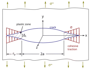
• EPFM is needed when the crack tip plastic zone is not negligible – i.e. significant plastic yielding happens before or during crack growth. In EPFM, linear elasticity no longer suffices, so we use other fracture parameters. The two main ones are J-integral and CTOD (Crack Tip Opening Displacement). The J-integral, introduced by Rice, represents a path-independent measure of energy available for crack growth (even with plasticity). CTOD, popularized by Wells, measures the physical opening displacement at the crack tip at the moment of fracture. Interestingly, it’s been shown that for a given material and conditions, J and CTOD are related – they’re two sides of the same coin. EPFM analysis often involves plotting a resistance curve (R-curve) of J or CTOD versus crack extension, or using a Failure Assessment Diagram (FAD) approach to account for both fracture and plastic collapse. Modern FEA software can directly calculate J-integrals for 3D cracks in ductile materials. For example, you might perform an EPFM simulation to determine if a crack will grow in a pressure vessel that experiences some plastic yielding at operating pressure. You’d look at J vs.J_{IC}
  (the material’s critical J toughness) or simulate the crack extension using a plastic damage model.

 

In summary, use LEFM (K, G) for brittle or small-scale yielding cases, and use EPFM (J, CTOD, damage models) when dealing with ductile behavior. Many simulation workflows start with LEFM for conservative estimates, then move to EPFM if needed for more accuracy once yielding is expected. For instance, ASME code guidance might say to use LEFM for initial screening, but if your crack is in a low-toughness material or the component sees plastic load, you switch to EPFM analysis.

Simulation Workflows: Modeling Cracks and Running Fracture Analyses

Now that we have the concepts down, let’s discuss how we simulate cracks in practice. Several software tools are widely used in industry for fracture mechanics: here we’ll look at Abaqus, Ansys, COMSOL Multiphysics, and a specialized tool Zencrack. Each has its own workflow for crack modeling, applying loads, defining material fracture properties, and interpreting results. I’ll outline what it’s like to use each, and then we’ll compare their capabilities.

Before diving in, note that in any simulation workflow, some common steps include:

1. Geometry and Crack Definition: Build the part geometry and introduce a crack (or crack-like flaw). This could mean an actual cut in the mesh, a seam, an initial notch, or an “enriched” crack region depending on the software.
2. Material Properties: Input properties including elastic modulus, Poisson’s ratio, and crucially fracture properties (e.g. K_{IC} , fatigue crack growth constants, or a material damage law). For ductile materials you might input a stress-strain curve and a J-integral resistance curve or cohesive zone parameters.
3. Meshing: Mesh the model with refinement near crack tips. Some tools have special crack tip elements or singularity elements; others use automated adaptive meshing.
4. Boundary Conditions & Loading: Apply loads or displacements representing the service conditions (tension, pressure, cyclic loading, etc.). For crack growth simulation, define the loading history (e.g. how many cycles, load amplitude).
5. Analysis & Crack Propagation: Run the analysis. Depending on the tool, the crack may remain stationary (to calculate K or J), or it may automatically grow a small amount if a criterion is met (like ΔK exceeding a threshold per cycle, or J exceeding J_{IC}).
6. Post-processing: Extract results – typically SIFs (K), energy release rates (G), J-integrals, or crack extension per cycle. We interpret these to see if the crack will grow, and if so, how fast and in what direction. Visualization of the crack path and stress distribution is also important.

Let’s see how our four tools handle these steps.

Abaqus (SIMULIA): Fracture Mechanics in a General-Purpose FEA

Abaqus is a powerful general FEA package, and it has extensive fracture mechanics capabilities. Users can model cracks in Abaqus in a few ways:

• XFEM (Extended Finite Element Method): Abaqus allows crack modeling without explicitly meshing the crack faces, by using XFEM. You designate an “enriched region” where a crack can grow, and Abaqus will handle the discontinuities in the displacement field internally. This is great for when you don’t know the crack path in advance (e.g. a crack could kink). Abaqus supports arbitrary crack initiation and growth with XFEM, though in some cases you might need a user subroutine or plugin to fully automate fatigue crack growth via XFEM. (Recent versions have improved built-in XFEM features for fracture.)
• Discrete crack with remeshing or node release: Alternatively, you can explicitly mesh a crack (say, a slit or an initial crack front in 3D) and then either allow it to grow by local remeshing or by node release techniques. In older workflows, one might partition the geometry for the crack and use the Virtual Crack Extension method or contour integrals to compute K and then advance the crack manually step by step.
• Cohesive zone modeling (CZM): Abaqus also permits inserting cohesive elements (with a traction-separation law) along potential crack paths. This is more of a damage-mechanics approach where the crack “grows” when the cohesive material fails. It’s often used for adhesive joints or composite delamination but can be applied to simulate ductile tearing as well.

Abaqus has a rich material library and allows defining failure criteria. For example, you can specify a fracture toughness in terms of energy (for use with a VCCT – Virtual Crack Closure Technique – or contour integral) or a cohesive energy for cohesive elements. You can also implement custom crack growth criteria. Abaqus is known for its robust solvers and the ability to handle complex models, but it can have a steep learning curve when setting up crack simulations.

Workflow in Abaqus: Suppose we want to model fatigue crack growth in a steel plate with a hole. We could either (a) use XFEM: define an enriched zone around the hole and let Abaqus initiate a crack when a stress criterion is met, or (b) introduce a pre-crack and use a cycle-by-cycle approach. In either case, we’d mesh the region finely. We’d apply cyclic loading (maybe via an amplitude curve). If using XFEM, we define a damage initiation (e.g. a maximum principal stress criterion) and a damage evolution law (fracture energy). Abaqus would then simulate crack initiation and propagation without us manually changing the mesh. We’d request output like History of contour integrals (to get K or J at each step) or the crack length as a function of cycles.

One of Abaqus’s strengths is the ability to combine fracture with other phenomena – e.g. you can run a thermomechanical fatigue crack growth simulation (maybe the crack grows faster in a hot section due to reduced toughness). You can script and automate runs to increment the crack length and compute life. Researchers have even written plug-ins for automated fatigue crack growth in Abaqus, since out-of-the-box Abaqus might require some user intervention for true fatigue life predictions.

Abaqus also supports multiple cracks and complex 3D crack geometries, but sometimes the setup requires careful partitioning or using its plug-ins (like the Crack feature in Abaqus/CAE for planar cracks). It is known for its computational efficiency and has options like parallel processing and adaptive remeshing to improve crack growth simulation speed.

In summary, Abaqus is extremely powerful but can be complex to set up. It provides both fracture mechanics-based criteria (stress intensity, energy release) and damage-based criteria (like cohesive models) for crack simulation. Many academic and industry studies use Abaqus for crack growth and have shown good correlation with experiments in areas like adhesive joint failure, composite cracking, and metal fatigue.

Ansys Mechanical: SMART Crack Growth and Fracture Tools

ANSYS has developed a very user-friendly workflow for fracture mechanics in its Workbench interface. A standout feature in recent versions is called SMART Crack Growth in Ansys Mechanical. “SMART” stands for Separating, Morphing, Adaptive, Re-meshing Technology – which is a fancy way of saying it automates crack growth with mesh updates. Here’s how Ansys handles cracks:

• You can insert a pre-defined crack in your model (Workbench has a crack tool where you specify location, size, and orientation of an initial crack or flaw). For example, you might insert a semi-elliptical surface crack in a pipe or a through-crack in a plate.
• Once the crack is defined, SMART Crack Growth takes over for simulation. ANSYS uses an Unstructured Mesh Method (UMM) to locally remesh around the crack front with tetrahedral elements as the crack advances. This greatly reduces manual meshing effort – historically, crack growth required lots of re-meshing, but ANSYS automates it and can cut what used to take days of meshing into minutes.
• The user specifies the crack growth parameters: it can handle fatigue crack growth (by inputting Paris law constants C, m, and perhaps a threshold ΔK) or static stable tearing (using fracture toughness and an incremental approach). ANSYS will then increment the crack, recalculating the mesh each step. It refines the mesh at the crack tip using a “sphere of influence” to ensure accuracy.
• Importantly, Ansys can simulate mixed-mode cracks and even multiple cracks simultaneously. The SMART feature will let multiple crack fronts grow in the same analysis, which is useful for complex structures that might have several flaws.
• Loading and criteria: For fatigue, ANSYS uses the classic Paris law approach: you give it ΔK vs da/dN info (or simply C, m) and it uses the stress intensity range from each analysis step to compute how much to extend the crack. For static loading, it can use a criterion like the J-integral or critical K to advance the crack until some instability criterion. In fact, ANSYS can do both static and fatigue crack growth in the same framework (static growth might be based on a critical energy release rate or K, and fatigue on Paris law).
• Results: Ansys provides SIF calculations (K values) and J-integral calculations as outputs. The user can see how K evolves as the crack grows, or how many cycles have elapsed. The simulation can stop automatically if, say, the crack reaches a certain length or if K exceeds K_{IC} (unstable fracture).

One cool aspect of ANSYS’s SMART approach is it will automatically handle crack initiation and arrest – meaning if the driving force falls, it can stop crack growth in the simulation. It also has cohesive zone capabilities: as the crack grows, new crack faces can have cohesive behavior applied, which can simulate things like crack closure or bridging forces.

From a usability perspective, ANSYS Workbench makes a lot of this quite graphical. For instance, to set up a crack growth analysis, you drop in a “Crack” object in the Simulation tree, define the crack (location, shape), then drop in a “SMART Crack Growth” object where you specify whether it’s fatigue or static, the material properties for crack growth (Paris constants or fracture toughness), and how many increments or cycles to simulate. The interface guides you through it, so you don’t have to manually script remeshing or anything.

Under the hood: ANSYS is doing a lot – VCCT, XFEM, and CZM are all available. Actually, ANSYS offers the Virtual Crack Closure Technique for computing energy release, and XFEM as well (especially for crack initiation problems). But the SMART feature is a more automated high-level tool that uses those techniques behind the scenes. It’s optimized for Mode I dominant cracks (opening mode), which covers many common cases (like cracks in pressure vessels or aircraft skins). The documentation notes some limitations: for example, it currently supports 3D crack growth, not 2D, and primarily Mode I (with some mixed Mode I/II).Also, the user needs to ensure the material data (Paris law constants, etc.) are accurate and that the mesh is sufficiently refined near the crack tip for reliable results.

Overall, ANSYS Mechanical has become a very strong tool for fracture mechanics that is relatively easy to use. It’s great for engineers who want to do a crack propagation study without writing custom scripts. I’ve seen it used for things like simulating a crack in a rotor shaft under cyclic torsion or analyzing a crack in a pipeline under pressure fluctuations. In one case, an engineer was able to simulate multiple load cycles and crack growth in an aerospace fitting and pinpoint when it would need repair – all within the ANSYS Workbench environment, which automatically took care of the heavy lifting of remeshing and cycle counting.

(One more thing: ANSYS also allows importing crack growth data for specific materials; e.g., NASGRO or FCG datasets can be used if you have them, rather than a simple Paris law. This can improve accuracy for regime I and III behaviors beyond Paris’ linear region.)

COMSOL Multiphysics: Flexibility for Fracture and Coupled Physics

COMSOL Multiphysics is known for its flexibility, especially if you need to couple fracture with other physics (like thermal, fluid, etc.). While COMSOL might not be as specialized in fracture as Zencrack or as out-of-the-box automated as ANSYS, it provides robust tools for Linear Elastic Fracture Mechanics and even some innovative methods like phase-field for cracks.

Key features of fracture simulation in COMSOL:

• J-integral and Stress Intensity Factors: COMSOL can directly compute SIFs using the J-integral method. The software has built-in contour integrals that allow you to calculate K_{I}, K_{II}, K_{III}
• for a given crack in a model. For instance, COMSOL’s documentation shows an example of a plate with an edge crack where they determine K_{I} via J-integral and energy release rate, and even compute the crack growth rate using Paris’ law. This means you can set up a stationary crack model, get the SIF, and then estimate how many cycles would grow the crack by a certain amount.
• Crack Modeling: In COMSOL, you typically define a crack by partitioning the geometry (like drawing a cut) or using special crack features. There’s a Fracture Mechanics Module (or part of the Structural Mechanics Module) which provides a “Crack” feature. For a 3D model, you can define an edge crack or an internal crack by specifying the crack front and crack plane. COMSOL will then create the geometry of the crack surfaces. You often mesh the crack surfaces with special elements. The software can handle multiple crack fronts too (though each might need to be defined).
• Material properties and models: COMSOL shines in allowing custom material behaviors. You can easily incorporate a Paris’ law for fatigue by writing an ODE or using its Fatigue Module. It also lets you include environmental or thermal effects – for example, you could have the material fracture toughness or fatigue properties depend on temperature, and simultaneously solve the heat transfer problem. COMSOL supports various material models (elastic-plastic, creep, etc.) which can be important if you do EPFM or time-dependent crack growth. You can input fracture toughness values, fatigue crack growth curves, or even implement a user-defined crack growth law if Paris’ law isn’t sufficient.
• Phase Field and Damage Methods: In recent years, COMSOL added capabilities for phase-field fracture, which is a method to simulate crack initiation and growth without explicitly tracking a crack surface. Instead, a diffused crack “phase” field evolves, splitting the material when it reaches a critical value. This is particularly useful for brittle fracture in complex shapes (like ceramic components or glass) where crack paths are not known in advance. COMSOL’s Phase Field fracture can be coupled with other physics (for example, simulate a piezoelectric material cracking while also solving the electric field).
• Multiphyics coupling: The big advantage of COMSOL is in scenarios like stress corrosion cracking, thermomechanical fatigue, or hydrogen-assisted cracking – basically, where you have more than just mechanical loading. COMSOL can couple mechanical stress with chemical diffusion or thermal expansion, etc. For example, you could simulate a crack in a pipeline steel where hydrogen concentration is high at the crack tip (making it more brittle), by coupling a diffusion equation with the fracture mechanics equation. Or consider fracture in electronic components: you might couple thermal cycling, creep, and cracking.

In terms of ease-of-use: COMSOL’s GUI is quite user-friendly for setting up standard LEFM analyses. It has an Application Library with examples like Single Edge Crack (which computes K and uses Paris law to find cycles to failure). These can be a template for your own analyses. You do have to manually set up crack growth increments if doing step-by-step propagation (unless using phase-field, which will propagate the crack naturally as part of the solution). There isn’t an automated crack growth increment loop in the GUI like ANSYS has, but you can script it with the Parametric Sweep or via the Fatigue Module. Essentially, COMSOL might require a bit more manual or scripting effort to simulate a crack growing over many increments – but in return, it gives you a lot of control and coupling capability.

For example, I once used COMSOL to simulate a crack in a polymer component where the crack growth rate depended on temperature. I set up a model where a transient thermal analysis ran (with cycles of heating and cooling), and at certain intervals I calculated the SIF and advanced the crack length based on Paris law using a little Java (MATLAB) snippet in COMSOL’s methods. It was a bit involved, but it allowed exploring how faster thermal cycles vs slower ones affected the crack growth – something that combined heat transfer and fracture in one go.

Another COMSOL case: analyzing a welded steel structure for fracture. One could import weld residual stresses (maybe from an initial simulation) and include those in the fracture analysis (residual stresses contribute to the stress intensity). COMSOL can include an initial stress field and compute SIF with that included. This is useful for e.g. predicting crack growth in a welded pressure vessel with residual stresses from welding.

Overall, COMSOL is like the Swiss army knife. It might not have dedicated automated crack growth wizards, but it provides the fundamental tools: J-integral calculations, material flexibility, and multiphysics. It is well-suited for R&D or complex problems (like coupling fracture with corrosion, etc.), and it’s quite capable for classical fracture problems too (with the added benefit that you can precisely define crack geometry and get accurate K solutions).

Zencrack: A Specialized Tool for Crack Growth (Often Used with Abaqus)

Zencrack is a bit different from the others – it’s a specialized fracture mechanics software focused on crack growth simulations. It’s not a general FEA tool by itself; rather, it works in conjunction with FEA solvers (especially Abaqus, and also ANSYS, MSC Nastran, etc.). Think of Zencrack as an automation and mesh-adaptation engine for crack propagation problems.

Key points about Zencrack:

• Integration with FE Solvers: Zencrack reads finite element models (e.g. an Abaqus input file) that contain an initial crack definition, and then it drives the crack growth by calling the FE solver iteratively. For example, you provide a cracked model in Abaqus, Zencrack computes SIFs along the crack front, decides how to advance the crack, modifies the mesh (or uses a special crack-block element approach), and then calls Abaqus for the next step. This loop continues for multiple crack growth increments. Zencrack essentially automates the fatigue crack growth simulation for you. It also has a plug-in for Abaqus/CAE to help set up Zencrack analyses.
• Crack Growth Criteria: Zencrack can handle both fatigue and static crack growth. For fatigue, you typically give it a crack growth law (Paris law or more advanced, even the NASGRO equation) and a loading schedule. It calculates ΔK (or ΔJ) along the crack front, figures out how the crack will advance (how much and in what direction at each point along the front) and then extends the crack. It supports mixed-mode growth and can advance cracks in arbitrary 3D orientations. One limitation noted in literature is that Zencrack assumes a predefined crack plane/front shape and doesn’t easily allow crack turning out of that initial plane – so if a crack wants to change direction sharply, you might need to reorient the model or use multiple cracks to approximate a curved path. However, Zencrack is quite capable of growing multiple crack fronts simultaneously and even letting them merge if needed.
• Meshing: Historically, a pain in crack growth simulation is meshing around the crack, especially after it grows. Zencrack uses a concept of crack-blocks in the mesh – basically partitioned meshes around the crack that it regenerates as the crack grows. It doesn’t have its own mesh generator for the whole model; instead, you prepare your model mesh with these crack blocks (like a template around the crack area), and Zencrack refines/regenerates those as needed. It relies on the host FEA code’s solver for the analysis portion.
• Applications and advantages: Zencrack is very popular in the aerospace industry and others where crack growth must be studied in detail (e.g. engine components, airframe structures). It’s also used in nuclear and offshore industries. One advantage is that it can consider complex loading sequences (spectrum loading, etc.) more easily and do automated crack growth over many cycles, outputting the crack shape evolution. It also allows multiple initial defects in a model – e.g. you could put multiple cracks in different locations and simulate them growing at the same time, to see which one becomes critical first or if they coalesce.
• Ease of use: Zencrack is more niche, and using it typically requires more knowledge of fracture mechanics. You often work with input text files, although there are GUI helpers. It’s not as drag-and-drop as ANSYS Workbench, but it’s extremely powerful for the specialist. It comes with an array of SIF solutions and routines for different geometries. Zencrack can consider things like residual stresses, thermal stresses, complex load combinations in crack growth – you can feed in results from an FE analysis and it will include the effect of those secondary stresses on crack growth.

One example: an engineer used Zencrack with Abaqus to predict crack growth in a bridge roller bearing under cyclic loading. The workflow was: build an Abaqus model of the bearing with an initial crack, then let Zencrack iterate – it took Abaqus results, computed SIFs, advanced the crack, remeshed, and repeated. The result was a predicted crack path and life that helped explain the failure that had been observed. Zencrack provided a flowchart of how it interacts with Abaqus (essentially a loop of solve -> crack advance -> solve). Another use case is in pipeline and riser analysis: Zencrack (and its sister product Zenriser) can simulate a crack growing in a pressurized riser pipe over time, including the effect of internal pressure and external loads.

Zencrack vs. doing it directly in Abaqus or Ansys? The benefit of Zencrack is that it’s highly specialized and optimized for fracture mechanics. It has many crack-growth specific features (like auto-adjusting the increment size if the crack is accelerating, etc.). However, it’s not as widely known or used as the mainline FEA programs – usually it’s fracture analysts who use it. In terms of ease-of-use, Zencrack requires learning its specific syntax and possibly some trial and error in setting up the crack-block mesh. Documentation is good but not as glossy as ANSYS/COMSOL. One could say Zencrack focuses on crack behavior more than anything else. If you have one job – simulate this crack growing – Zencrack is built for that. Whereas Abaqus or Ansys are more general platforms that also do crack growth.

A limitation to note: Zencrack doesn’t generate the initial mesh – you need an FE model ready. It also doesn’t do non-FE stuff (no CFD, etc.). So it’s a specialist add-on, which is why many companies pair “Zencrack + Abaqus”. Abaqus provides the general FE muscle, Zencrack provides the crack growth brains.

To highlight a real-world scenario: Consider a pipeline with a longitudinal seam weld crack. An analyst might use Zencrack to grow that crack under pressure cycling and occasional water hammer loads. They could include weld residual stresses in the initial condition. Zencrack would take the combined stress state, compute SIFs along the long crack front (which might be semi-elliptical), and propagate it a small amount per load cycle block. They could see the crack shape evolve (perhaps growing deeper into the wall and longer along the pipe). The output might tell them after how many cycles the crack will reach critical size. This kind of analysis could certainly be done in Ansys or COMSOL too, but Zencrack provides pre-built routines for a lot of it, possibly making it more efficient and proven in safety-critical industries. In fact, aerospace tends to trust such specialized tools that have been validated on numerous crack growth problems.

Comparing the Software Platforms

Now that we’ve looked at each tool, how do they stack up against each other? The choice often comes down to the specific needs of your project:

• Capability: All four can calculate stress intensity factors and simulate crack propagation, but their methods differ. Zencrack is highly specialized for crack growth, with advanced options for fatigue laws and proven accuracy on 3D crack fronts. Abaqus and Ansys are general FEA with strong fracture features – Abaqus offers more manual control and variety of methods (XFEM, cohesive, etc.), while Ansys offers streamlined automated crack growth (SMART) especially for Mode I cracks. COMSOL provides flexibility and multiphysics – great if your crack problem isn’t just mechanical (thermal, corrosive environment, etc.).
• Ease of Use: Ansys Mechanical likely wins here for typical industrial users – its GUI-driven crack setup (SMART Crack Growth) is very user-friendly, and you don’t need to be a crack expert to get results. COMSOL is also GUI-oriented and fairly intuitive for setting up basic fracture analyses (plus it has good tutorials), but doing advanced crack propagation might need some scripting. Abaqus has a steeper learning curve; setting up a crack in Abaqus/CAE is doable (especially 2D cracks), but advanced tasks often require writing Python scripts or using command files. Zencrack requires expertise – it’s typically used by fracture specialists. You have to prepare an input deck and understand crack-block strategy, which is a barrier for new users. In short: if you want quick results and have a straightforward task (like a single crack in a part under cyclic load), Ansys might get you there fastest. If you’re doing a research-heavy or unusual simulation, Abaqus or COMSOL give you more freedom. And if your company routinely analyzes crack growth in critical parts, investing in Zencrack makes sense.
• Integration and Workflow: Zencrack is integrated with Abaqus (and others) but that means you’ll be juggling two programs. Abaqus and Ansys are each self-contained (one GUI/solver to manage). COMSOL is self-contained too and shines when you need to integrate different physics. If you already have a lot of Abaqus know-how or models, using Abaqus for fracture (possibly with Zencrack add-on) is logical. If you’re an ANSYS shop, the new crack growth tools there are plenty capable.
• Accuracy and Validation: All these tools, when properly used, can produce accurate results that match experimental data. For example, publications have compared them: one study compared ABAQUS, FRANC3D, ZENCRACK, and others for fatigue crack growth and found each has strengths – Zencrack and Franc3D were very accurate for pure fracture mechanics tasks, while Abaqus needed more user intervention but is very robust, and ANSYS’ automated features greatly improved user efficiency. Ansys’s SMART crack growth has been verified on standard test cases (like crack growth in compact tension specimens). Abaqus has decades of use in fracture research (with many papers using Abaqus for crack modeling). COMSOL’s results for K and J have been verified against handbook solutions and other FEA. The key is often the user’s expertise: garbage in, garbage out. Setting up boundary conditions correctly (especially for fracture problems, e.g. ensuring Mode I vs Mode II mix is right) is crucial regardless of software.
• Special Features: Abaqus has the unique capability of XFEM for arbitrary 3D crack paths and a rich material model library (for example, you can simulate ductile crack initiation with a damage model like Gurson or Johnson-Cook damage in Abaqus). Ansys has the automated meshing and multiple crack handling in an easy package, plus both 2D and 3D crack options. COMSOL can do phase-field without manual meshing of cracks, which is cutting-edge for brittle fracture simulation (like crack patterns in concrete or ceramics). Zencrack can handle multiple growing cracks and complex crack geometries out-of-the-box, and it’s known to handle combined loads and even time-dependent crack growth (like creep crack growth) if needed.

To help decide: If someone asks “Zencrack vs Abaqus for crack growth modeling?”, the answer might be: use Zencrack with Abaqus if you need an industry-validated, automated crack growth solution for a complex 3D problem and have the time to invest in setup – this combo is used in aerospace and nuclear a lot. If the question is “Ansys vs Abaqus for fracture?”, and the context is a company doing routine fracture assessments, Ansys Workbench is easier to get started and integrate with other Ansys workflows (like if you already do stress analysis in Workbench, adding crack growth is simple). Abaqus might be chosen for more advanced or nonstandard analyses, or if the company already has Abaqus licenses and expertise. For multiphysics or customized research problems, COMSOL might be the choice due to its flexibility.

Real-World Applications and Case Studies

It’s all well and good to talk theory and software features, but what about real-world engineering scenarios? Fracture mechanics simulation is heavily used in several industries:

• Oil & Gas (Pipelines and Pressure Vessels): Imagine a long oil pipeline where a flaw exists in a weld. Fracture simulations help predict if that crack will grow due to pressure cycles (say, daily start-up/shutdown) or remain stable. Engineers use tools like Abaqus or Ansys to calculate stress intensity along such a longitudinal weld crack. They might simulate crack propagation using Paris’ law to estimate remaining life. As an example, one could simulate a crack in a pipeline’s girth weld under internal pressure fluctuations – if the Paris law constants for the pipe steel are known, the software can predict crack growth per year. Fitness-for-service assessments (per standards like BS 7910 or API 579) often require such analysis but doing it via simulation gives more detailed insight (like how the crack shape might evolve, not just if it will fail). In a high-pressure gas vessel, fracture simulation might be used to set safe operating limits: e.g., determine the critical crack size at operating pressure by finding when K = K_{IC} . In one project, a high-pressure waterbox (part of a power plant heat exchanger) with multiple embedded cracks was analyzed in stages: a global model provided loads to a submodel with a crack, and crack growth was simulated to ensure it wouldn’t propagate through the wall. This helped avoid unnecessary shutdowns by showing the cracks were stable under transients.
• Aerospace (Aircraft Structures, Engines): The aerospace sector arguably has the most rigorous fracture control requirements. Simulation is used to certify that cracks will not grow to failure between inspection intervals. For instance, consider a crack in an airplane wing skin near a fastener hole – an analyst might use Zencrack or Franc3D with Abaqus to propagate the crack under flight load spectra, ensuring it doesn’t reach a critical length. Or in jet engines, tiny cracks in turbine discs are assessed with crack growth simulation because temperatures are high and materials are specialty alloys. The simulations incorporate the Paris law with an elevated-temperature correction or use da/dN data from lab tests at high temp. Aerospace also leverages damage tolerance analysis, where tools like Zencrack shine in assessing crack growth under complex multi-axial stress states.
• Nuclear Industry: Nuclear reactors and their components (like reactor pressure vessels, piping, and steam generator tubing) use fracture mechanics to ensure safety. Here, elastic-plastic fracture is often important (due to ductile materials operating near brittle-ductile transition temperatures). A classic case: the reactor pressure vessel must be analyzed for a pressurized thermal shock scenario – a rapid cooling that could cause a crack to propagate brittlely. Fracture simulation (often with Abaqus or specialized codes) would calculate the stress intensity during the transient and compare to material toughness (which is temperature-dependent). Another example is welded components in nuclear plants: they often have residual stresses and operate for decades, so predicting if a detected flaw will grow is crucial. Simulations may incorporate weld residual stress fields (maybe imported from a weld modeling analysis) and then do a crack growth analysis. Codes like ASME Section XI guide these assessments, but simulation allows a more nuanced look (like the actual 3D crack front shape changes). In one study, a team used Abaqus with a user subroutine to simulate fatigue crack growth in a reactor nozzle, capturing the effect of cladding and residual stress – something analytical formulas alone would struggle with.
• Structural and Mechanical Engineering: Fracture mechanics pops up in many other areas – from analyzing the cracks in large bridges, to failures in rotating machinery, to even consumer electronics (drop tests causing glass cracks). Wherever there’s a risk of crack initiation and growth, these simulation tools can help. For example, a welded crane hook might undergo fracture simulation to ensure a crack that initiated from a weld defect won’t grow under repeated lifts. Or a railway axle might be simulated for crack growth under rolling contact fatigue. Another interesting application: additively manufactured (3D-printed) metals often have different defect characteristics, so engineers are using simulation to study how cracks initiate from voids or lack-of-fusion defects. COMSOL’s multiphysics ability could, for instance, couple thermal stresses from the printing process with a fracture analysis to see if a crack would start upon cooldown.

Each industry often has its preferred tools: Oil & gas and power generation folks might lean towards Ansys or Abaqus (sometimes with in-house tools or spreadsheets using standards). Aerospace and high-end mechanical often use Abaqus + crack growth utilities (Zencrack, Franc3D) or specialized codes like NASGRO for simpler analyses. But increasingly, these distinctions blur as all the major software improve – many companies use a bit of everything, cross-validating the results.

What’s important is that in all cases, the simulations must be validated against either analytical solutions or experiments. The stakes are high when predicting fractures (nobody wants to be the engineer who underestimates a crack growth and has a pipeline rupture or a plane grounded!). Thankfully, the combination of classical fracture mechanics formulas and modern FEA gives engineers multiple ways to double-check their work.

Conclusion: Choosing the Right Tool and Best Practices

Fracture mechanics may sound intimidating, but I hope this walkthrough has made the core ideas clearer. We talked about how stress intensity factors indicate crack driving force, how cracks grow under cyclic loads as described by Paris’ law, and how materials can fail in a brittle or ductile manner (necessitating either LEFM or EPFM analysis). These concepts are the backbone of any fracture simulation, whether you use Abaqus, Ansys, COMSOL, or Zencrack.

When it comes to choosing software for fracture mechanics simulation or crack growth modeling, consider the following:

• For routine industrial problems (single cracks, known locations): Ansys Mechanical’s SMART Crack Growth can be a quick and reliable choice. It provides an engineer-friendly interface to set up cracks and get results without deep scripting. It’s especially good if you’re mostly dealing with fatigue cracks in metals and need to evaluate life or inspect intervals.
• For advanced or research problems: Abaqus offers unparalleled depth – you can simulate almost any fracture process if you know how to tweak it. It’s great for EPFM (ductile tearing simulations, etc.) and complex 3D crack interaction problems. Coupling with Zencrack further enhances Abaqus for automated fatigue crack growth. If your crack path is unknown or you expect crack kinking, Abaqus XFEM is very useful.
• For multiphysics or customized scenarios: COMSOL might be the best, since you can include thermal effects, fluids, chemical degradation, etc., all in one model. It might also be easier for educational use, given its intuitive UI for setting up things like J-integrals and crack geometries.
• For multiple cracks or life prediction of systems: Zencrack (or similar tools like FRANC3D) are tailored for crack propagation in complex structures with high fidelity. They often plug into your existing FEA workflows (like using your Abaqus models) and add crack-specific smarts. These are worth it if crack growth is a recurring concern in your work (for example, if you’re tasked with managing a fleet of assets with cracks, or doing damage tolerance analysis regularly).

A big takeaway is that all simulations must be grounded in good data and engineering judgment. That means: use correct material properties (get those fracture toughness values, Paris law constants from lab tests or literature), apply realistic loads and boundary conditions, and whenever possible, correlate your simulation with a known solution or a test. For instance, if you can measure crack growth in a prototype, do it and compare with your model – it builds confidence.

Fracture mechanics can save the day by predicting failures before they happen, but only if used correctly. The software tools we discussed are just that – tools. An experienced engineer will use them in combination. It’s not unusual to do a quick hand calc (using, say, API 579 formulas or NASGRO library solutions) to estimate a crack’s life, and then do a detailed FEA simulation to refine the understanding of the crack behavior. The detailed simulation might reveal things the simple calc missed – like maybe the crack will turn towards a stiffener, reducing the driving force, thus giving a longer life than the hand calc predicted. These insights are incredibly valuable for making informed decisions about repairs, inspection, or design modifications. For more information among fracture mechanics check our related webinar and online course!

Finally, if you’re dealing with a critical fracture problem and need help, it’s wise to consult with experts or use reputable services. As an expert in this field, I’ve seen how a fresh perspective or advanced simulation can pinpoint solutions that extend a component’s life or avoid catastrophic failure. Our team at Engineering Downloads is always ready to assist with fracture simulations – whether it’s setting up a Zencrack model for a pipeline defect, running an Abaqus EPFM analysis for a pressure vessel, or using COMSOL to couple fracture with other effects. Feel free to reach out if you have a challenging crack problem; we’re here to help turn fracture mechanics theory into practical, safe engineering outcomes.