Understanding Damage Modeling in Engineering Simulations
In the world of engineering, preventing component failure is paramount. Whether you’re designing an aircraft wing, a pipeline, or a medical implant, understanding how materials degrade and eventually fail under various loads is critical. This is where damage modeling comes in – a powerful computational approach that helps engineers predict and analyze the progressive deterioration of materials before complete fracture.
Damage modeling is an essential aspect of modern structural integrity assessments, moving beyond simple yield criteria to provide a more realistic picture of a component’s remaining life and ultimate failure. It’s particularly vital in fields like structural engineering, aerospace, oil & gas, and biomechanics, where safety and reliability are non-negotiable.

Damage model visualization in a steel component, illustrating stress concentration and potential failure zones. Image courtesy of Wikimedia Commons.
Why Damage Modeling is Crucial for Engineers
Traditional strength-of-materials approaches often rely on simplified assumptions or empirical data, which might not fully capture complex failure mechanisms like progressive softening, void growth, or micro-cracking. Damage modeling offers a more detailed and predictive capability, allowing engineers to:
- Predict Material Degradation: Understand how properties like stiffness, strength, and toughness evolve as damage accumulates.
- Assess Structural Integrity: Evaluate the remaining useful life of components under cyclic, impact, or sustained loading.
- Optimize Designs: Identify critical areas susceptible to damage and reinforce them, leading to lighter, stronger, and more durable products.
- Simulate Complex Failure Modes: Accurately represent ductile fracture, brittle failure, and even delamination in composites.
- Enhance Safety: Provide a higher level of confidence in designs, especially for safety-critical applications like pressure vessels or aircraft structures (e.g., FFS Level 3 assessments).
Fundamentals of Damage Mechanics
At its core, damage mechanics describes the material’s response as microscopic defects (voids, cracks, dislocations) nucleate, grow, and coalesce. These micro-scale events lead to a macroscopic reduction in the material’s load-bearing capacity.
Continuum Damage Mechanics (CDM)
CDM treats damage as a continuous internal variable, typically represented by a scalar or tensor damage variable (D). This variable reflects the effective loss of cross-sectional area or stiffness. As D increases from 0 (undamaged) to 1 (fully damaged/fractured), the material’s elastic modulus and strength degrade. Most commercial FEA software, like Abaqus and ANSYS Mechanical, implement various CDM models.
Key Concepts in CDM:
- Effective Stress Concept: Relates the applied stress to an “effective” stress that acts on the undamaged portion of the material.
- Damage Evolution Law: Defines how the damage variable grows based on plastic strain, stress triaxiality, temperature, and other factors.
- Damage Initiation Criteria: Specifies the conditions under which damage begins to accumulate.
Micromechanics-Based Models
These models attempt to explicitly link macroscopic damage evolution to specific microstructural phenomena, such as void nucleation and growth in ductile materials. A prime example is the Gurson-Tvergaard-Needleman (GTN) model, which tracks the void volume fraction and its influence on macroscopic yield behavior and softening. While more computationally intensive, GTN offers a deeper physical insight into ductile fracture processes.
Fracture Mechanics vs. Damage Mechanics
It’s important to distinguish damage mechanics from traditional fracture mechanics. Fracture mechanics focuses on the propagation of pre-existing macroscopic cracks using concepts like stress intensity factors or J-integrals. Damage mechanics, on the other hand, models the initiation and growth of damage zones that precede macroscopic cracking, often leading to the prediction of crack initiation and subsequent propagation without explicitly defining an initial crack.
Key Material Models for Damage Prediction
Selecting the right damage model is crucial and depends heavily on the material, loading conditions, and the failure mechanism you’re trying to capture. Here are some common categories:
Ductile Damage Models
These models are suitable for materials that exhibit significant plastic deformation before failure, like many metals. They often link damage evolution to plastic strain and stress state.
- Johnson-Cook Damage Model: Widely used for high strain rate applications (e.g., impact, crashworthiness). It’s typically coupled with the Johnson-Cook plasticity model and defines damage initiation based on equivalent plastic strain, stress triaxiality, and strain rate.
- Gurson-Tvergaard-Needleman (GTN) Model: As mentioned, GTN is excellent for modeling void growth and coalescence in ductile metals, particularly when stress triaxiality plays a significant role in failure. It requires careful calibration but provides robust predictions for phenomena like necking and ductile fracture.
- Lemaitre-Chaboche Model: A classic CDM model that defines damage evolution based on equivalent plastic strain and stress.
Brittle Damage Models
For materials that fail with little to no plastic deformation (e.g., ceramics, concrete, some composites, cast iron), brittle damage models are more appropriate. These often rely on stress or strain limits.
- Max Principal Stress/Strain Criterion: Simple models where damage initiates when the maximum principal stress or strain reaches a critical value. Often used as a first approximation.
- Cohesive Zone Models (CZM): Not strictly a continuum damage model, CZM simulates crack initiation and propagation by introducing a “cohesive zone” ahead of a crack tip. This zone represents the progressive separation of material interfaces and is defined by a traction-separation law. CZMs are powerful for modeling delamination in composites or crack growth in quasi-brittle materials.
- Concrete Damaged Plasticity (CDP): Specific to concrete, this model captures both tensile cracking and compressive crushing, incorporating distinct damage variables for tension and compression.
Fatigue Damage Models
When components are subjected to cyclic loading, fatigue damage can accumulate over time, leading to eventual failure even at stresses below the material’s yield strength. Fatigue damage modeling can be approached in several ways:
- Stress-Life (S-N) Approach: Empirical method linking stress amplitude to cycles to failure, often used for high-cycle fatigue.
- Strain-Life (ε-N) Approach: More suitable for low-cycle fatigue, relating plastic strain amplitude to cycles to failure.
- Crack Propagation Models (e.g., Paris Law): Utilized when an initial crack is assumed, predicting its growth under cyclic loading.
- Abaqus/ANSYS Built-in Fatigue Tools: Integrate S-N or ε-N curves with FEA results to predict fatigue life based on stress/strain histories.
Composite Damage Models
Composites present unique challenges due to their anisotropic nature and multiple failure modes (fiber fracture, matrix cracking, delamination). Dedicated models are needed, often involving multiple damage variables or criteria, such as Hashin criteria, LaRC, or Puck criteria, coupled with cohesive zone models for delamination.
Comparison of Common Damage Models
Choosing the right damage model can significantly impact your simulation’s accuracy and computational cost. Here’s a brief overview:
| Damage Model Type | Typical Materials | Primary Failure Mode | Complexity & Calibration | Common Software Support |
|---|---|---|---|---|
| Johnson-Cook | Ductile metals (e.g., steels, aluminum) | Ductile fracture, high strain rate | Moderate; requires flow stress & damage parameters from tests (tension, shear, notched) | Abaqus/Explicit, ANSYS Explicit Dynamics, LS-DYNA |
| Gurson-Tvergaard-Needleman (GTN) | Ductile metals with void growth | Ductile fracture (void nucleation, growth, coalescence) | High; extensive calibration needed for void parameters | Abaqus, ANSYS Mechanical |
| Cohesive Zone Models (CZM) | Brittle/quasi-brittle (e.g., composites, concrete, adhesive joints) | Crack initiation & propagation, delamination | Moderate; requires traction-separation law parameters (fracture energy, peak traction) | Abaqus, ANSYS Mechanical, Nastran |
| Concrete Damaged Plasticity (CDP) | Concrete, masonry | Tensile cracking, compressive crushing | Moderate; specific parameters for tension/compression damage evolution | Abaqus, ANSYS Mechanical |
Practical Workflow for Damage Modeling in FEA
Implementing damage models effectively requires a structured approach within your CAD-CAE workflow. Here’s a typical progression:
Step 1: Define Objectives and Failure Modes
Before diving into simulation, clearly identify:
- What type of failure are you trying to predict (e.g., ductile fracture, brittle cracking, fatigue, delamination)?
- What are the critical loads and environmental conditions?
- What level of accuracy is required?
This guides your choice of damage model and material characterization efforts.
Step 2: Material Characterization and Parameter Calibration
This is often the most challenging part. Damage models rely on specific parameters (e.g., fracture energy, critical plastic strain, void nucleation parameters). These are typically obtained through:
- Experimental Testing: Tensile tests (with varying stress triaxiality via notched specimens), shear tests, compact tension tests, or specific fracture tests.
- Inverse Modeling: Simulating the experimental tests and adjusting material parameters until the simulation matches the experimental force-displacement or load-displacement curves. Tools like Abaqus, ANSYS, and specialized material characterization software often have features for this.
- Literature Review: Leveraging published data for similar materials, though caution is advised due to material variability.
Step 3: Model Setup in FEA Software
Using software like Abaqus or ANSYS Mechanical, set up your geometry and mesh as you would for any nonlinear analysis. Ensure your material model includes the chosen damage criterion and evolution law.
- Defining Damage: In Abaqus, this might involve defining “Damage for Ductile Metals,” “Damage for Fiber-Reinforced Composites,” or “Cohesive Behavior.” In ANSYS, you might use Explicit Dynamics material models or specific commands for damage accumulation.
- Element Type: Choose elements capable of handling large deformations and potential element deletion, if that’s part of your damage model’s strategy. Reduced integration elements (e.g., C3D8R in Abaqus) are common.
Step 4: Meshing Considerations
Mesh density is critical, especially in regions prone to damage initiation and propagation. Damage models are often sensitive to mesh size, as energy dissipation can be path-dependent.
- Fine Mesh in Critical Zones: Ensure sufficient element density where damage is expected.
- Regularity: Strive for a relatively structured and regular mesh to avoid artificial stress concentrations.
- Mesh Independence Studies: Essential to confirm that your results are not overly dependent on your mesh size (see Verification section).
Step 5: Boundary Conditions and Loading
Apply realistic boundary conditions and loading sequences that reflect the real-world scenario. Ensure your loading path matches the experimental conditions used for material characterization.
Step 6: Solver Settings and Convergence
Damage modeling often involves severe nonlinearities. Configure your solver settings appropriately:
- Nonlinear Geometry: Always enable large deformation/nonlinear geometry settings.
- Automatic Time Stepping: Use automatic time incrementation to help the solver navigate difficult convergence points.
- Explicit vs. Implicit: For highly dynamic events with severe damage (e.g., impact, crash), explicit solvers (e.g., Abaqus/Explicit, LS-DYNA) are often preferred due to their robust handling of element deletion and large deformations. For quasi-static problems, implicit solvers are more common, but convergence can be challenging.
If you’re looking to tackle complex damage modeling projects or need high-performance computing resources, EngineeringDownloads offers affordable HPC rental, specialized online courses, and expert project consultancy.
Verification & Sanity Checks for Damage Models
Ensuring the reliability of your damage model results is paramount. Don’t just trust the numbers – verify them!
Mesh Sensitivity Analysis
Run your simulation with several different mesh densities, especially in the damage-prone regions. Observe if the predicted damage initiation, evolution, and final failure load change significantly. If results vary wildly with mesh refinement, your model might be mesh-dependent and require further refinement or regularization techniques (e.g., element length-dependent damage parameters).
Boundary Condition (BC) and Loading Review
Double-check all applied loads and constraints. An incorrectly applied BC can drastically alter stress distributions and damage predictions. Visualize reactions and displacements to confirm they are physically reasonable.
Energy Balance and Mass Conservation (Explicit Solvers)
For explicit dynamic analyses, monitoring the energy balance (internal energy, kinetic energy, external work, artificial strain energy) is crucial. High artificial strain energy can indicate poor mesh quality or instability. Also, ensure mass conservation if elements are being deleted.
Comparing with Simple Analytical Models or Hand Calculations
Even for complex damage scenarios, simple checks can provide sanity. Can you estimate the ultimate tensile strength or rupture energy based on simplified mechanics? Does your model at least capture the qualitative behavior correctly?
Experimental Validation (Conceptual)
While you might not perform experiments yourself, remember that robust damage models are ideally validated against experimental data. If your organization has access to test results, comparing simulation predictions (e.g., force-displacement curves, crack patterns) with experiments is the gold standard.
Sensitivity Analysis of Material Parameters
Explore how sensitive your results are to small variations in your damage parameters. Since these parameters often have some uncertainty, understanding their impact on the outcome helps in assessing the robustness of your predictions. Python scripts often aid in automating these parametric studies.
Common Pitfalls and Troubleshooting in Damage Modeling
Damage modeling is powerful but comes with its own set of challenges. Here’s what to watch out for:
Element Deletion Issues
Many damage models use element deletion as a way to simulate material separation. However, premature or excessive element deletion can lead to:
- Loss of Stiffness: If too many elements are deleted, the structure can become artificially soft.
- Numerical Instability: Sudden changes in stiffness can cause convergence problems.
- Unrealistic Crack Paths: Element deletion follows mesh lines, which might not represent the physical crack path.
Troubleshooting: Carefully review the damage initiation and evolution parameters. Consider using cohesive elements or XFEM if explicit crack representation is critical and element deletion is problematic.
Convergence Difficulties
Nonlinearities from plasticity and damage accumulation can make implicit solutions difficult to converge.
- Troubleshooting: Reduce increment sizes, adjust solver controls (e.g., number of cutbacks), check for singularities from contact or boundary conditions, and ensure good element quality. For severe problems, consider switching to an explicit solver if appropriate for the physics.
Material Parameter Calibration Challenges
Getting accurate damage parameters often requires significant effort and specialized experimental data.
- Troubleshooting: Invest in high-quality experimental data. Utilize inverse modeling techniques. Be cautious with parameters taken directly from literature without proper validation for your specific material and processing.
Overly Complex Models
Resist the temptation to use the most advanced damage model if a simpler one suffices. Model complexity increases computational cost and calibration effort.
- Troubleshooting: Start simple, validate, and then incrementally add complexity only if necessary to capture observed phenomena.
Industry Applications of Damage Modeling
Damage modeling is invaluable across various engineering disciplines:
Aerospace Engineering
Predicting crashworthiness of aircraft structures, assessing impact damage on composite wings, simulating fatigue life of landing gear components, and understanding delamination in laminated materials. Tools like Abaqus, LS-DYNA, and MSC Nastran are heavily utilized here.
Oil & Gas and Structural Engineering
Critical for assessing the structural integrity of pipelines, pressure vessels, offshore platforms, and other infrastructure. Damage modeling supports Fitness-for-Service (FFS Level 3) assessments, predicting crack initiation and growth under operating conditions, and analyzing ductile fracture risks. It helps in life extension decisions and risk management.
Biomechanics
Simulating the failure of bones, tissues, and medical implants under physiological loads. Understanding how prosthetics interact with bone, or how tissue responds to injury, benefits greatly from damage mechanics. FEA tools coupled with patient-specific CAD models are common.
Automotive Industry
Crash simulations, occupant safety, fatigue analysis of chassis components, and predicting material failure in vehicle structures during impact events. Explicit dynamic solvers are the workhorse in this domain.
Advanced Topics and Future Trends
The field of damage modeling continues to evolve rapidly:
- Extended Finite Element Method (XFEM): Allows cracks to propagate independently of the mesh, offering advantages in complex crack path predictions without remeshing.
- Peridynamics: A non-local continuum theory that naturally handles crack initiation and propagation without needing explicit crack tracking algorithms, particularly useful for highly discontinuous problems.
- AI/Machine Learning: Emerging applications involve using ML to accelerate material parameter calibration, predict damage evolution, or even develop new constitutive models directly from experimental data. Python and MATLAB are frequently used for developing these advanced algorithms.
- Multi-scale Modeling: Linking atomic, micro-scale, and macro-scale damage phenomena to create more predictive and physically accurate models.
Further Reading
For more in-depth information on continuum damage mechanics, a foundational text is “Continuum Damage Mechanics for Engineering Materials” by Lemaitre and Chaboche. You can also explore specific software documentation for detailed implementations of damage models, such as the Abaqus Documentation on Damage and Failure.
Conclusion
Damage modeling is an indispensable tool in the modern engineer’s toolkit. It moves beyond traditional safety factors to offer a sophisticated, predictive capability for understanding how materials and structures degrade under load. While challenging, with careful model selection, robust material characterization, and diligent verification, damage modeling provides invaluable insights that lead to safer, more efficient, and more reliable engineering designs. Mastering these techniques is a significant step towards becoming a top-tier simulation engineer.