Ductile Damage Analysis: From Theory to FEA Simulation

Ductile Damage
Engineering Downlaods
March 9, 2026
17 Minute

Ductile damage is a fundamental failure mechanism that engineers encounter across nearly all industries, from aerospace to oil & gas. Unlike brittle fracture, where a material fails suddenly with little prior deformation, ductile materials exhibit significant plastic deformation before ultimate failure. Understanding, predicting, and mitigating ductile damage is paramount for ensuring product safety, extending operational lifespans, and optimizing structural designs. This article delves into the core concepts of ductile damage, its modeling using Finite Element Analysis (FEA), and practical considerations for robust simulations.

$Micrograph showing the dimpled surface characteristic of ductile fracture in steel.$

Scanning Electron Micrograph (SEM) of a ductile fracture surface, revealing characteristic dimples.

Understanding Ductile Damage: The Basics

At its heart, ductile damage involves the progressive degradation of a material’s load-carrying capacity due to the formation and growth of microscopic voids. This process is typically observed in metals and polymers that can undergo substantial plastic deformation.

What is Ductile Fracture?

Ductile fracture is a complex multi-stage process characterized by three main phases:

Void Nucleation: Microscopic voids form at interfaces between the matrix and second-phase particles (like inclusions or precipitates) or at grain boundaries. This often happens under localized stress concentrations during plastic straining.
Void Growth: As plastic deformation continues, these nascent voids grow and expand under the influence of macroscopic plastic flow and hydrostatic stress (stress triaxiality).
Void Coalescence: The growing voids eventually link up, often through the formation of micro-void sheets in the material between larger voids, leading to the formation of macro-cracks and ultimate failure.

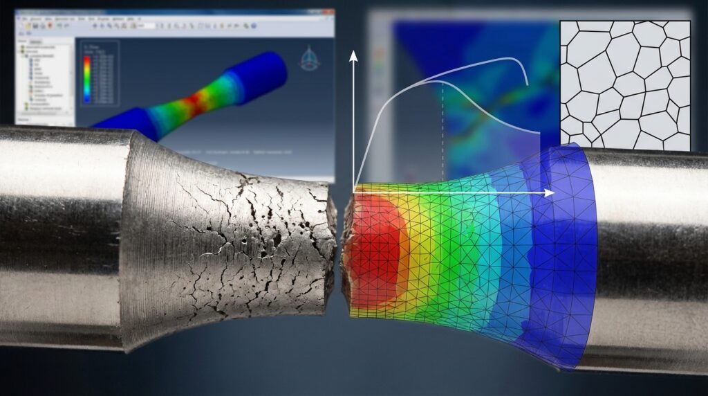
The macroscopic result is typically a fracture surface with a characteristic ‘dimpled’ appearance, indicating the pulling apart of the material around the voids.

Why is it Important in Engineering?

The ability of materials to deform plastically before fracture is often a desirable trait, as it provides a warning of impending failure and allows for energy absorption. However, uncontrolled ductile damage can lead to:

Premature Component Failure: Structures can fail below their designed ultimate strength.
Reduced Service Life: Damage accumulation can lead to faster degradation and fatigue.
Safety Concerns: Catastrophic failures in critical components (e.g., pipelines, aircraft structures, pressure vessels) can have severe consequences.
Economic Impact: Costly repairs, downtime, and potential litigation.

For structural engineers, particularly in fields like Oil & Gas (Fitness-for-Service Level 3 assessments) and Aerospace, accurately predicting ductile damage is crucial for reliable design and integrity management.

Key Mechanisms of Ductile Damage

Delving deeper into the mechanics helps in selecting appropriate damage models and interpreting simulation results.

Void Nucleation

Void nucleation is often initiated by the decohesion of inclusions from the matrix or the cracking of brittle particles within the ductile matrix. The presence, size, shape, and distribution of these particles significantly influence when and where voids begin to form. Higher stress triaxiality (the ratio of hydrostatic stress to equivalent von Mises stress) can accelerate nucleation.

Void Growth

Once nucleated, voids grow primarily due to the bulk plastic deformation of the surrounding material. Stress triaxiality plays a critical role here; a high triaxial stress state (e.g., at the tip of a notch or crack) promotes void expansion, while shear stress favors elongation and potential coalescence through shear banding. The rate of void growth is typically a function of accumulated plastic strain and stress state.

Void Coalescence

The final stage, void coalescence, occurs when neighboring voids link up to form a continuous crack. This can happen in two primary ways:

Internal Necking: The material ligaments between larger voids plastically neck down and rupture.
Shear Localization: Micro-voids form in shear bands between larger voids, creating a path for crack propagation. This mechanism is common under lower stress triaxiality conditions.

The specific mode of coalescence influences the macroscopic fracture path and overall toughness.

Material Models for Ductile Damage

Simulating ductile damage in FEA requires specialized material models that can account for the initiation and evolution of damage. These models typically couple plastic deformation with damage accumulation.

Phenomenological Models

These models describe the macroscopic behavior of materials experiencing ductile damage without explicitly modeling individual voids. They are widely used in commercial FEA software like Abaqus, ANSYS Mechanical, and MSC Nastran due to their computational efficiency and practical applicability.

Gurson-Tvergaard-Needleman (GTN) Model: This is one of the most widely recognized and implemented ductile damage models. It incorporates a void volume fraction as an internal state variable, which evolves with plastic strain and stress triaxiality. GTN can capture nucleation, growth, and coalescence, and it’s effective for porous ductile materials. Key parameters include initial void volume fraction, nucleation strain, and parameters controlling void growth and coalescence.
Johnson-Cook Damage Model: Often coupled with the Johnson-Cook plasticity model for high strain rate applications, this model defines damage initiation based on accumulated plastic strain, strain rate, and temperature. Damage evolution is then typically controlled by a fracture energy criterion, leading to element deletion or stiffness reduction. It’s popular in crashworthiness (automotive) and impact simulations.
Lemaitre-Chaboche Damage Model: This model views damage as a scalar variable that reduces the effective stress-carrying area of the material. Damage evolves as a function of plastic strain and is often combined with isotropic or kinematic hardening plasticity models. It’s versatile but can be challenging to calibrate.

Choosing the Right Model

The selection of a ductile damage model depends on several factors:

Material Type: Some models are better suited for specific material classes (e.g., metals vs. polymers).
Loading Conditions: High strain rates (Johnson-Cook), quasi-static (GTN, Lemaitre).
Available Experimental Data: The ability to calibrate the model’s parameters is crucial. Uniaxial tensile tests, notched tensile tests, and shear tests are common for calibration.
Computational Cost: Simpler models are faster, but more complex models may offer higher accuracy for specific phenomena.

Practical Workflow for Ductile Damage Simulation (FEA)

Implementing ductile damage models in FEA requires a structured approach to ensure accuracy and reliability. Here’s a typical workflow:

1. Material Characterization

This is arguably the most critical step. Accurate material parameters are essential. You’ll need:

Uniaxial Tensile Test Data: Stress-strain curve (true stress-true strain) up to fracture.
Notched Tensile Tests: To introduce varying stress triaxiality and calibrate void growth/coalescence parameters.
Shear Tests: To capture material behavior under low triaxiality conditions.
Fracture Toughness Data: Provides a benchmark for the material’s resistance to crack propagation.

Tools like Python or MATLAB can be invaluable for post-processing raw test data and performing inverse calibration of damage model parameters.

2. Model Setup in FEA Software

Geometry & Meshing: Import your CAD model. For damage simulations, use continuum elements (e.g., C3D8R in Abaqus, SOLID186 in ANSYS) that support damage. Local mesh refinement is crucial in areas where damage is expected to initiate and propagate. Damage models are highly mesh-sensitive.
Material Properties: Input your plasticity model (e.g., isotropic hardening) and then the chosen ductile damage model parameters (e.g., GTN parameters, Johnson-Cook parameters).
Boundary Conditions & Loading: Apply realistic constraints and loads that mimic the actual service conditions. Consider both magnitude and rate of loading.

3. Damage Initiation & Evolution

Define how damage initiates and evolves within your chosen FEA software:

Initiation Criterion: Specify the condition for damage to begin (e.g., a critical plastic strain, stress triaxiality threshold, or void volume fraction).
Evolution Law: Define how damage progresses after initiation, typically by gradually reducing the material’s stiffness or defining a critical equivalent plastic displacement at which elements are removed or deactivated (element deletion).

4. Solving the Simulation

Ductile damage simulations are highly non-linear and often require advanced solver settings:

Implicit vs. Explicit: For quasi-static problems, an implicit solver (e.g., Abaqus/Standard, ANSYS Mechanical) with appropriate non-linear solution controls might be used. For highly dynamic events (e.g., impact), explicit solvers (e.g., Abaqus/Explicit, ANSYS Autodyn) are generally more robust for handling large deformations and element deletion.
Convergence: Be prepared for convergence difficulties due to stiffness degradation and element deletion. Adjust increment sizes, use stabilization techniques, or consider alternative solution strategies.

Common Pitfalls

Mesh Sensitivity: Damage models are notorious for producing mesh-dependent results. A finer mesh often leads to earlier damage initiation and propagation. Careful mesh sensitivity studies are essential.
Parameter Calibration: Incorrectly calibrated damage parameters will yield inaccurate predictions. This often requires iterative comparison with experimental data.
Numerical Stability: Element deletion can lead to sudden changes in stiffness and convergence issues.

If you’re looking to run complex ductile damage simulations, EngineeringDownloads offers affordable HPC rental to power your models, alongside online courses and project consultancy to enhance your team’s expertise.

Verification & Sanity Checks for Ductile Damage Models

Even with the best models and parameters, thorough verification and validation are critical for confidence in your results.

Mesh Sensitivity Analysis

Perform simulations with at least three different mesh densities (coarse, medium, fine) in critical damage zones. Analyze key outputs like fracture initiation location, peak load, and displacement at failure. Ideally, results should converge with mesh refinement, though total energy absorbed might be a more stable metric than displacement for highly localized failure.

Boundary Condition & Loading Checks

Visually inspect the deformed mesh and reaction forces to ensure boundary conditions are applied as intended and loads are distributed realistically. Simple static checks or hand calculations can confirm initial load distributions.

Convergence Criteria

Monitor the solver’s convergence history (e.g., force residuals, energy balances). A well-converged solution indicates that the numerical solution is stable. Divergence or sudden jumps in residuals often signal issues with material properties, contact, or time stepping.

Qualitative & Quantitative Validation

Qualitative: Does the damage initiation location and propagation path align with physical intuition or experimental observations?
Quantitative: Compare simulation results (e.g., load-displacement curves, displacement at fracture, energy absorption) against experimental data or validated benchmarks. Discrepancies often point to material model calibration issues or incorrect damage parameters.

Parameter Sensitivity Analysis

Vary individual damage model parameters (e.g., GTN nucleation strain, Johnson-Cook critical plastic strain) within reasonable bounds to understand their impact on the simulation results. This helps identify the most influential parameters and quantify the robustness of your model’s predictions.

Applications Across Engineering Disciplines

The principles and simulation techniques for ductile damage are widely applicable:

Oil & Gas and Structural Integrity (FFS Level 3)

Assessing the integrity of aging pipelines, pressure vessels, and offshore structures. Ductile damage models help predict the remaining life and potential failure modes of components containing defects or operating under severe conditions. FFS Level 3 assessments heavily rely on advanced non-linear FEA incorporating damage.

Aerospace Components

Designing lightweight yet robust aircraft structures. Ductile damage analysis is crucial for predicting crack initiation in fuselage panels, wings, and engine components, improving fatigue life, and ensuring crashworthiness.

Automotive Safety

Optimizing vehicle crashworthiness. Simulating the deformation and failure of energy-absorbing structures (e.g., crumple zones) during impacts to enhance occupant safety. Johnson-Cook models are frequently used here.

Biomechanics (e.g., bone fracture)

While often considered brittle, bone and other biological tissues can exhibit ductile-like damage mechanisms at micro-scales. Damage models assist in designing implants, predicting bone fracture under impact, or understanding tissue degradation.

Troubleshooting Common Ductile Damage Simulation Issues

Simulating ductile damage can be challenging. Here are some common problems and troubleshooting tips:

Premature Element Deletion / Excessive Distortion

Check Material Properties: Ensure stress-strain curves are smooth and accurately extrapolated.
Review Damage Parameters: If parameters are too low, damage initiates too early.
Mesh Quality: Highly distorted elements can lead to solver abortion. Check element quality and consider adaptive meshing.
Stabilization: Add artificial damping or viscous regularization if available in your solver to improve stability.

Lack of Convergence / Aborts

Time Incrementation: Reduce initial and minimum time increments.
Non-Linear Solution Controls: Adjust settings like maximum number of iterations, residual tolerances.
Contact Issues: Unstable contact definitions can cause divergence. Ensure proper contact properties and stabilization.
Material Definition: Discontinuities in material response (e.g., sudden softening) can be problematic.

Unrealistic Damage Progression

Re-calibrate Parameters: This is the most common cause. Compare against more experimental data.
Mesh Sensitivity: Confirm your mesh is fine enough but not excessively sensitive.
Boundary Conditions: Are they truly representing the physical constraints?
Model Choice: Is the selected damage model appropriate for the material and loading?

Ductile Damage Model Parameters: An Illustrative Example

Here’s a simple, illustrative table of typical parameters you might encounter for a Gurson-Tvergaard-Needleman (GTN) damage model. Note that actual values are highly material-specific and must be calibrated from experimental data.

Parameter	Description	Typical Range (Illustrative)	Impact on Damage
f₀ (Initial Void Volume Fraction)	Initial porosity of the material.	0.0001 – 0.01	Higher f₀ means earlier damage.
q₁, q₂, q₃ (Tvergaard Parameters)	Modify void growth rate based on stress triaxiality.	q₁=1.5, q₂=1.0, q₃=2.25	Influence void shape evolution and growth.
ε_n (Nucleation Strain)	Plastic strain at which new voids begin to nucleate.	0.1 – 0.5 (dimensionless)	Lower ε_n means earlier nucleation.
f_N (Nucleation Void Volume Fraction)	Void volume fraction of newly nucleated voids.	0.001 – 0.05	Controls the amount of new porosity introduced.
S_N (Standard Deviation of Nucleation Strain)	Spreads out the nucleation process over a strain range.	0.05 – 0.1	Larger S_N means gradual nucleation.
f_c (Critical Void Volume Fraction)	Void fraction at which void coalescence initiates.	0.1 – 0.3	Lower f_c means earlier coalescence.
f_F (Final Void Volume Fraction)	Void fraction at final rupture/element deletion.	0.15 – 0.5	Higher f_F means more ductile failure before full rupture.

Frequently Asked Questions (FAQs)

What is the primary difference between ductile and brittle fracture?

Ductile fracture involves significant plastic deformation (e.g., necking, void formation) before failure, absorbing a lot of energy. Brittle fracture, conversely, occurs with little to no plastic deformation, often propagating rapidly and absorbing less energy.

Why is stress triaxiality so important in ductile damage models?

Stress triaxiality (the ratio of hydrostatic stress to von Mises stress) profoundly influences void growth. High triaxiality promotes void expansion and accelerates damage, making materials appear less ductile, while low triaxiality often favors shear-dominated failure mechanisms.

Can I use linear elastic FEA to analyze ductile damage?

No, linear elastic FEA cannot capture ductile damage. Ductile damage is inherently a non-linear phenomenon that involves plastic deformation and material degradation, requiring non-linear material models and advanced solver capabilities available in non-linear FEA software.

How do I calibrate ductile damage model parameters for my material?

Calibration typically involves performing a series of experimental tests (e.g., uniaxial tensile, notched tensile, shear tests) on your material. The force-displacement data from these tests are then used, often through inverse modeling techniques and optimization algorithms (sometimes scripted in Python or MATLAB), to determine the unique parameters that best fit the experimental observations.

What are the challenges of simulating ductile damage with FEA?

Key challenges include mesh sensitivity of results, accurate calibration of complex material model parameters, numerical convergence issues due to material softening and element deletion, and the need for significant computational resources, especially for large, dynamic models.

Is element deletion always the best way to model ductile fracture?

Element deletion is a common and often effective approach for modeling the final separation of material. However, it can lead to mesh dependency and loss of overall force equilibrium. Alternative methods, such as cohesive zone models (CZM) or eXtended Finite Element Method (XFEM), can provide more robust crack propagation modeling without explicit element removal, especially when dealing with complex crack paths.