Welcome to the world of Computational Fluid Dynamics (CFD)! If you’re an engineer looking to understand fluid flow, heat transfer, and related phenomena without relying solely on expensive and time-consuming physical experiments, CFD is your powerful ally. This tutorial provides a practical, engineer-to-engineer guide to mastering CFD, from setting up your first simulation to validating your results.
Fluid dynamics impacts nearly every aspect of engineering, from aircraft design and pipeline efficiency to biomedical devices and urban air quality. CFD transforms complex differential equations into solvable algebraic equations, allowing us to predict fluid behavior with remarkable accuracy.

Airflow simulation around an airfoil, demonstrating typical CFD output.
The Power of CFD: Why Engineers Use It
CFD is more than just a simulation tool; it’s a strategic asset for design, analysis, and optimization. Here’s why it’s indispensable:
- Design Optimization: Quickly iterate through design variations to find optimal shapes for minimal drag, maximum lift, or efficient mixing.
- Performance Prediction: Accurately predict how a system will behave under various operating conditions before physical prototyping.
- Cost Reduction: Significantly reduce the need for expensive physical prototypes and experiments.
- Insight into Physics: Visualize complex flow patterns, pressure distributions, and temperature gradients that are difficult or impossible to observe experimentally.
- Troubleshooting: Diagnose and resolve performance issues in existing systems.
Understanding the CFD Workflow: A Step-by-Step Guide
A typical CFD analysis follows a structured process. Mastering each step is key to reliable results.
Step 1: Define Your Problem and Geometry
Before any simulation, clearly define the engineering problem you’re trying to solve. What are the objectives? What data do you need?
- Problem Statement: Clearly articulate the physical phenomena you want to study (e.g., pressure drop across a valve, heat transfer in a heat exchanger, aerodynamic drag on a vehicle).
- Geometry Acquisition/Creation: Obtain or create the 3D model of your system. This often involves CAD software like CATIA, SolidWorks, or Inventor. Simplify the geometry by removing minor features that don’t significantly impact the fluid flow but would complicate meshing.
- Fluid Domain Definition: Extract the fluid volume from your CAD model. This is the region where the fluid will flow and where the simulation will be performed.
Step 2: Mesh Generation (Discretization)
Meshing divides your fluid domain into a large number of small, discrete cells (elements). The quality and density of this mesh critically impact the accuracy and computational cost of your simulation.
- Mesh Types: Common types include structured (hexagonal) and unstructured (tetrahedral, polyhedral, prismatic/wedge) meshes. Polyhedral meshes, for example, offer good balance between accuracy and computational cost.
- Mesh Refinement: Areas with high gradients (e.g., near walls, wakes, inlets/outlets) require finer meshes to capture flow details accurately.
- Boundary Layer Meshing: Special attention is needed near walls to resolve the viscous sub-layer using prism layers or inflated boundary layers, crucial for accurate wall shear stress and heat transfer predictions.
- Tools: Software like ANSYS Meshing, Pointwise, or OpenFOAM’s
snappyHexMeshare used for this step.
Step 3: Setting Up the Physics and Boundary Conditions
This is where you tell the solver what physics to simulate and how the fluid interacts with its surroundings.
- Governing Equations: Specify the relevant equations (e.g., Navier-Stokes for momentum, energy equation for heat transfer, species transport for chemical reactions).
- Fluid Properties: Define material properties (density, viscosity, thermal conductivity, specific heat) for your fluid. These can be constant or temperature/pressure dependent.
- Turbulence Model: For most real-world engineering flows, turbulence is present. Select an appropriate turbulence model (e.g., k-epsilon, k-omega, SST k-omega, LES, DES) based on the flow regime and desired accuracy vs. computational cost.
- Boundary Conditions (BCs): These define the conditions at the edges of your fluid domain:
Inlet:Specify velocity, pressure, mass flow rate, temperature.Outlet:Specify pressure (gauge), outflow, or a zero-gradient condition.Wall:Specify no-slip (fluid velocity is zero relative to the wall), slip, or heat transfer conditions (fixed temperature, heat flux, convection).Symmetry:Used to reduce computational domain for symmetric problems.
Step 4: Solving the Equations
With the geometry, mesh, and physics defined, the numerical solver begins to compute the flow field.
- Solver Settings: Choose appropriate numerical schemes (e.g., first-order upwind for stability, second-order upwind for accuracy) and pressure-velocity coupling algorithms (e.g., SIMPLE, PISO).
- Convergence Criteria: Define thresholds for residuals (measures of how well the equations are being satisfied). Typically, residuals should drop by several orders of magnitude (e.g., 1e-4 to 1e-6) and monitor quantities of interest (e.g., drag, lift, temperature) should stabilize.
- Iteration Process: The solver iteratively solves the discretized equations until convergence is achieved.
- Tools: Commercial software like ANSYS Fluent, ANSYS CFX, Siemens STAR-CCM+, or open-source solutions like OpenFOAM are commonly used.
Step 5: Post-Processing and Visualization
Once the simulation converges, you extract meaningful insights from the vast amount of data generated.
- Quantitative Analysis: Calculate performance metrics like pressure drop, drag coefficient, heat transfer rate, mass flow rate, etc.
- Qualitative Analysis: Visualize flow fields using contours (pressure, velocity, temperature), vectors (velocity direction), streamlines, and iso-surfaces to understand flow structures.
- Animations: Create dynamic visualizations for unsteady (transient) simulations.
Practical Workflow Considerations
Beyond the core steps, several practical aspects can streamline your CFD efforts.
CFD Software Landscape
The choice of software often depends on your budget, project complexity, and industry. Commercial tools like ANSYS Fluent/CFX and STAR-CCM+ offer extensive features, robust solvers, and excellent support, often integrated with CAD-CAE ecosystems. Open-source options like OpenFOAM provide flexibility and cost savings but require a steeper learning curve and more user responsibility for validation.
CAD-CAE Integration
Seamless integration between CAD (Computer-Aided Design) and CAE (Computer-Aided Engineering) tools is vital. Modern workflows allow direct transfer of geometry, reducing errors and saving time. Ensure your CAD models are clean and simplified before moving to the meshing stage.
Leveraging Scripting for Automation
Repetitive tasks in CFD, such as geometry modifications, mesh generation for parametric studies, or post-processing data extraction, can be automated using scripting languages like Python or MATLAB. This significantly speeds up the analysis process and reduces human error. Many CFD software packages offer scripting APIs. EngineeringDownloads.com provides downloadable scripts and templates for common CFD automation tasks, helping you streamline your projects!
Verification & Sanity Checks: Trusting Your Results
A beautiful contour plot doesn’t automatically mean your results are accurate. Rigorous verification and validation are crucial.
Mesh Independence Study
This is paramount. Perform simulations with progressively finer meshes and observe how your results for key quantities (e.g., drag coefficient, pressure drop) change. When further mesh refinement no longer significantly alters the results, you’ve achieved mesh independence. This confirms your solution is not overly dependent on the mesh resolution.
Convergence Criteria Check
Ensure that your residuals have dropped sufficiently and that the engineering quantities of interest have stabilized. Running for more iterations than necessary is inefficient, but stopping too early yields inaccurate results.
Validation Against Experimental Data or Analytical Solutions
Whenever possible, compare your CFD results with experimental data or known analytical solutions for simpler cases. This builds confidence in your model’s ability to predict real-world phenomena. Even qualitative comparisons (e.g., flow separation patterns) can be highly informative.
Sensitivity Analysis
Investigate how sensitive your results are to variations in input parameters like boundary conditions, material properties, or turbulence model choices. This helps understand the robustness of your predictions and identify critical inputs.
Common Pitfalls and Troubleshooting Tips
Every CFD engineer encounters challenges. Here are some common issues and how to address them.
Poor Mesh Quality
- Problem: Skewed elements, high aspect ratio cells, or insufficient resolution near critical areas.
- Fix: Improve mesh metrics using advanced meshing tools. Refine boundary layers, use local mesh sizing, and consider polyhedral or structured meshes where appropriate.
Incorrect Boundary Conditions
- Problem: Over-constraining the flow, under-constraining it, or applying conditions that don’t match the physical setup.
- Fix: Double-check all BCs against your physical problem. Ensure consistent units. Use appropriate outflow conditions (e.g., pressure outlet) that allow the flow to develop naturally.
Lack of Convergence
- Problem: Residuals oscillate or plateau at high values, and monitor quantities don’t stabilize.
- Fix:
- Check mesh quality.
- Relax under-relaxation factors (for steady-state) or reduce time step (for transient).
- Verify boundary conditions for physical realism.
- Simplify turbulence model initially (e.g., k-epsilon instead of SST k-omega) for stability.
- Examine solution domain for high velocities or challenging flow features.
Misinterpreting Results
- Problem: Believing quantitative results without qualitative checks or physical intuition.
- Fix: Always perform sanity checks. Do the results make physical sense? Are the pressure drops reasonable? Does the flow direction align with expectations? Visualize multiple variables (velocity, pressure, temperature) to get a complete picture.
Choosing the Right CFD Software
Selecting the appropriate software is crucial for efficient and accurate simulations. Here’s a brief comparison of popular options:
| Software | Type | Key Features | Pros | Cons | Typical Use Case |
|---|---|---|---|---|---|
| ANSYS Fluent | Commercial | Comprehensive physics models, advanced meshing, robust solver | Industry standard, extensive features, strong support | High cost, steep learning curve for full features | Aerospace, Automotive, Energy, Turbomachinery |
| ANSYS CFX | Commercial | Specialized for rotating machinery, efficient solver | Excellent for turbomachinery, fast convergence | Slightly less flexible for general-purpose fluid dynamics than Fluent | Pumps, Turbines, Compressors |
| OpenFOAM | Open Source | Command-line driven, highly customizable, C++ libraries | Free, highly flexible, large user community | Steep learning curve, less intuitive GUI, community support only | Academic research, specialized applications, cost-sensitive projects |
| Siemens STAR-CCM+ | Commercial | Integrated workflow, sophisticated meshing, multiphysics | Unified environment, excellent meshing automation | High cost, complex for beginners | Automotive, Marine, Industrial equipment |
Further Your CFD Journey
CFD is a vast and continuously evolving field. This tutorial provides a solid foundation. To truly master it, consistent practice, deep understanding of fluid mechanics principles, and continuous learning are essential. Experiment with different software, explore various applications, and never stop questioning your results.
For further in-depth knowledge and official documentation, refer to:
Further Reading: ANSYS Student CFD Resources