Different material behaviors

The material library in Abaqus provides a wide range of options for modeling various engineering materials, such as metals, plastics, rubbers, foams, composites, granular soils, rocks, plain and reinforced concrete, and also different material behavior models including elastic and plastic behavior. Material behaviors fall into the following general categories:

• general properties (material damping, density, thermal expansion);
• elastic mechanical properties;
• inelastic mechanical properties;
• thermal properties;
• acoustic properties;
• hydrostatic fluid properties;
• equations of state;
• mass diffusion properties;
• electrical properties; and
• Pore fluid flow properties.

A single material definition cannot combine certain mechanical behaviors because they are mutually exclusive. Additionally, certain behaviors necessitate the presence of others. For instance, plasticity requires the existence of linear elasticity.

Recently, we have discussed hyperelastic behavior as a subsection of elastic behavior (to see hyperelastic materials behavior content click here). At first, it would be better to study the general material behavior.
Typically, materials exhibit two distinct phases in their behavior as described by stress-strain curves: the elastic regime and the plastic regime.

Elastic regime

When external forces act upon a material, it can deform, but it can recover its original shape and size once the forces are no longer present. We refer to this ability as elastic behavior. In the elastic regime, the material undergoes temporary deformation, and the relationship between stress (force per unit area) and strain (deformation) is linear. Hooke’s Law describes the relationship between stress and strain within a material’s elastic limit, stating that stress is directly proportional to strain. The material exhibits instantaneous and reversible deformation during the elastic phase.

Plastic regime

Plastic behavior occurs when a material undergoes permanent deformation, even after the removal of external forces. Beyond the elastic limit, the material experiences significant strain without recovering its original shape and size. Additionally, it undergoes irreversible deformation. The stress-strain relationship in plastic deformation exhibits non-linearity, as stress increases along with strain. Factors such as crystal structure, movement of dislocations, and material defects influence the material’s capacity to undergo plastic deformation.

Elastoplastic behavior

Elastoplastic behavior combines elements of both elastic and plastic responses. In the elastoplastic regime, the material undergoes both elastic and plastic deformation. Initially, within the elastic limit, the material behaves elastically, exhibiting reversible deformation. As the applied stress surpasses the elastic limit, plastic deformation occurs. Consequently, there are permanent changes to the material’s shape. Many materials, including metals, commonly demonstrate elastoplastic behavior characterized by a linear elastic response initially, followed by plastic deformation. In this blog, we will delve into the behavior of materials in the plastic regime, and furthermore, we will explore the modeling of plastic materials.

In ABAQUS, various material models are available to describe the plastic behavior of materials. Here we are going to discuss metals and general materials plastic behavior models, and in the next blog, we will discuss Specialized Plasticity Models for Engineering Materials.

Plastic models in Abaqus

In ABAQUS, various material models are available to describe the plastic behavior of materials. Here is a list that explains commonly used material models.

Plastic

In the plastic section, in addition to providing stress-strain data for the plastic regime, it is also necessary to specify the method for determining hardening behavior. While users can define their custom model, they can also choose from predefined models such as isotropic, kinematic, multilinear, and Johnson-Cook models.

Isotropic hardening

This method assumes that the yield stress increases uniformly with plastic strain, regardless of the direction of loading. The isotropic hardening law defines a single parameter, which is the isotropic hardening modulus. The formulation for isotropic hardening is as follows:

σ = σy + K * εp

Where σ is the stress, σy is the initial yield stress, K is the isotropic hardening modulus, and εp is the plastic strain.

Kinematic hardening

Moreover, this method is based on the assumption that the yield stress increases with plastic strain in a direction parallel to the direction of loading. In addition, the kinematic hardening law is defined by two parameters: the kinematic hardening modulus and the back stress tensor. To elaborate, the formulation for kinematic hardening can be described as follows:

β = 1 – (2/3) * (K/Ks)

Where K is the kinematic hardening modulus and Ks is the saturation value of K 1.

A brief comparison

Let’s have a brief comparison of these two hardening methods: There are generally two types of material hardening behavior 2: one based on assumptions from monotonic tests and another based on real material response. The first type, called isotropic hardening, assumes that material yielding during unloading occurs when the stress range changes by twice the value of the highest stress reached prior to unloading (∆𝜎 = 2𝜎‘). This type of hardening assumes uniform hardening in all directions. On the other hand, kinematic hardening predicts that yielding in the reverse direction happens when the stress change from the unloading point is twice the monotonic yield stress (∆𝜎 = 2𝜎𝑜). Kinematic hardening behavior considers the Bauschinger effect (early yielding in compression) and is often more suitable for representing the actual behavior of cyclically loaded materials compared to isotropic hardening.

When comparing and indicating the difference between isotropic and anisotropic plastic behavior, researchers have demonstrated that the utilization of different plasticity models in the simulation of sheet metal forming can yield varying values for the predicted thickness of the blank, particularly in the case of anisotropic behavior.

Multilinear-kinematic hardening:

This method combines isotropic and kinematic hardening. It assumes that the yield stress increases with plastic strain in both isotropic and kinematic directions. Researchers have defined the multilinear-kinematic hardening law with three parameters: the isotropic hardening modulus, the kinematic hardening modulus, and the backstress tensor. The formulation of multilinear-kinematic hardening specifies the relationship and equations governing its behavior.

σ = σy + K * εp + β * b

The stress-strain behavior illustrated below demonstrates the initial response observed during the first four cycles of a material that undergoes cyclic hardening. In order to accurately simulate this behavior in finite element analysis (FEA), it is necessary to utilize a mixed-mode hardening model 3.

Johnson-Cook:

The Johnson-Cook model is a plasticity model that is based on Misses plasticity. It employs analytical equations to define the hardening behavior and the relationship between the strain rate and the yield stress 4. This method models strain rate and temperature effects on material behavior. It uses a power-law relationship to describe strain rate sensitivity and an exponential relationship to describe thermal softening. Since this material model is based on isotropic hardening, it cannot accurately predict the unloading response of many thermoplastics. The Johnson-Cook model has five parameters: A, B, n, C, and m. The formulation for Johnson-Cook hardening is the one that provides.

where A, B, n, C, and m are material constants, εp is the plastic strain, ε˙ is the strain rate, ε˙0 is a reference strain rate, T is temperature, and Tm is melting temperature.

Drucker-Prager/Cap Plasticity Model:

The purpose of this model is to simulate the behavior of cohesive geological materials, including soils and rocks, which have properties that change with pressure and can yield under certain conditions. To properly utilize this model, it is crucial to combine it with the CAP HARDENING feature. When performing an Abaqus/Standard analysis and considering creep material behavior, it is necessary to utilize the CAP CREEP option in conjunction. This criterion accounts for the permanent deformation of the material and can effectively consider both compaction and shear failure, including the transitional region between these two failure regimes.  It comprises of  three components. First, there is a linear shear failure surface that depicts the increasing shear stress with increasing mean stress, emphasizing shearing flow. Second, there is a curved “cap” that intersects both the shear failure surface and serves as an inelastic hardening mechanism to indicate plastic compaction. Lastly, there is the mean stress axis and a transition surface that enables a seamless intersection between the cap and failure surfaces. The equations that describe the three surfaces in the p-q plane, which represent equivalent pressure stress versus deviatoric stress, are expressed.

Shear failure surface,

The variable q represents the Von Mises equivalent stress or deviatoric stress measure, while p represents the hydrostatic pressure stress. The angle of friction is denoted by ϕ, and the material cohesion is represented by c.

Compression cap:

In this context, we define the smooth transition yield surface intersection between the cap and failure surfaces by utilizing the numeric parameter α. We denote the representation of the ratio between the horizontal axis and the vertical axis of the elliptical cap as R. Additionally, pa serves as an evolution parameter for volumetric plastic strain-driven hardening or softening of the cap.

Transition surface:

Consider the following alternative explanations below:

1. Material cohesion, d, within Abaqus/Standard, measures in the p–t plane, while in Abaqus/Explicit, it measures in the p–q plane. The units for measuring material cohesion are FL−2.

2. The material angle of friction, β, in Abaqus/Standard, is measured within the p–t plane. In Abaqus/Explicit, it is measured within the p–q plane. When entering the value, it should be in degrees.

3. Cap eccentricity parameter, R, determines the eccentricity of the cap. Its value should be greater than zero, typically ranging from 0.0001 to 1000.0.

4. Initial cap yield surface position, represented as εpvol||0, indicates the initial position of the cap’s yield surface.

5. Transition surface radius parameter, α, determines the radius of the transition surface. It should be a small value compared to unity. If left blank, the default is 0.0, indicating no transition surface. To include creep properties, you must set α to zero.

6. Flow stress ratio, denoted as K, represents the ratio of the flow stress in triaxial tension to the flow stress in triaxial compression. Its value should be between 0.778 and 1.0. In Abaqus, leaving it blank or entering 0.0 sets the default value of 1.0, except when creep properties are included, where you should set K to 1.0. This parameter applies only to Abaqus/Standard analyses.

7. Temperature.

8. Predefined field variables, referred to as Field n.

Concrete damaged plasticity

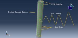
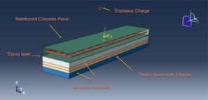
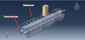
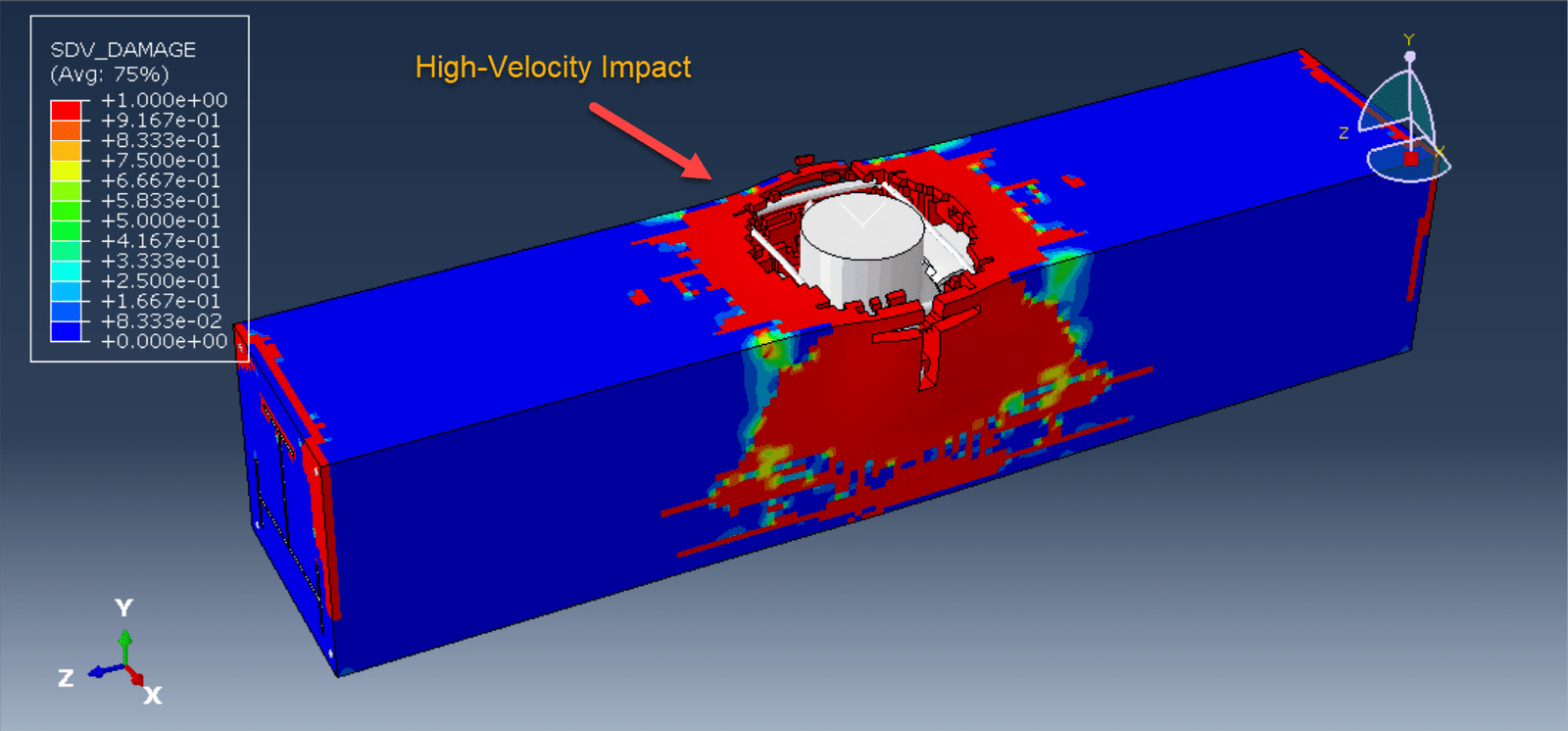
Concrete is a very heterogeneous material which shows complex nonlinear mechanical behavior. In addition, it is very difficult to define damage in a concrete structure. In the analysis of concrete structures using the finite element method, material models are used for these purposes. An example of these material models is concrete damage plasticity material model. This material model combines the yield theory of plasticity and theory of damage mechanics in order to effectively analyze the concrete structures behavior. The Abaqus concrete damaged plasticity model is a general tool for simulating the behavior of concrete and similar materials in various structural elements (such as beams, trusses, shells, and solids). This modeling approach combines isotropic damage mechanics and isotropic plasticity theory to accurately capture the inelastic deformation of concrete. Originally designed for reinforced concrete analysis, it also has the capability to handle plain concrete and effectively considers the presence of reinforcement bars embedded in the material. It can accommodate various loading conditions, including monotonic, cyclic, or dynamic loading, under low confining pressures. The approach utilizes a nonassociated multi-hardening plasticity model and a scalar damage model to accurately describe the irreversible damage caused by cracking.

Additionally, it provides users with control over stiffness recovery during cyclic loading and incorporates strain rate effects and viscoplastic regularization to enhance its performance, particularly in the softening regime. This comprehensive and adaptable approach offers improved accuracy and reliability in modeling and analyzing concrete behavior. The model assumes that the material has a linear and isotropic elastic response.

Yield function

The yield function of concrete damage plasticity material model is defined by equation:

Where:

The concept presented is a concrete model that considers the continuous deformation and damaging of the material. It acknowledges two primary ways in which the concrete can fail: cracking under tension and crushing under compression. The progression of the yield or failure surface is influenced by two hardening variables, labeled as εtpl and εcpl, which represent the equivalent plastic strains experienced by the material in tension and compression, respectively. The model describes the behavior of concrete under uniaxial tension and compression using damaged plasticity, as depicted in the figure below

When subjected to uniaxial tension, concrete exhibits a linear elastic relationship until it reaches the failure stress σt0. At this point, micro-cracking occurs within the material. As the stress exceeds the failure stress, the concrete’s response becomes softer, leading to strain localization throughout the structure. Conversely, under uniaxial compression, the response is initially linear until it reaches the initial yield stress σc0. In the plastic regime, the concrete exhibits stress hardening followed by strain softening beyond the ultimate stress σcu.

Although this representation is simplified, it captures the primary characteristics of how concrete behaves under different loading conditions.

Parameters

Also, it should be noted that in this model some parameters are asked which are described and explained here:

1. Dilation Angle: The dilation angle is a parameter in the plasticity model that determines the rate at which the volume of the concrete expands or dilates under shearing. In other words, it is a measure of how the volume of the concrete changes in response to shear stresses. This angle is typically determined from experimental data, and its value can have a significant impact on the predicted behavior of the concrete.
2. Eccentricity: The eccentricity in the concrete damaged plasticity model is a parameter that controls the shape of the yield surface in the model. This parameter affects the transition from the initial shape to the final shape of the yield surface as the concrete undergoes damage. The eccentricity parameter is usually calibrated using experimental data.
3. fb0/fc0: This parameter represents the ratio of the initial biaxial compressive yield stress (fb0) to the uniaxial compressive yield stress (fc0). It is used to define the shape of the yield surface. This ratio is typically obtained from experimental data.
4. K: K is the ratio of the second stress invariant on the tensile meridian to that on the compressive meridian at initial yield. It reflects the difference in behavior of concrete under tension and compression. This parameter is also typically obtained from experimental data.
5. Viscosity Parameter: The concrete damaged plasticity model incorporates the rate of loading into the model by utilizing the viscosity parameter. This becomes important for simulations where the rate of loading significantly differs from the rate at which the experimental data was obtained. A higher viscosity parameter will result in a slower response to loading.

Conclusion

In this blog, we embarked on a journey to explore the fascinating world of metals and general materials plastic behavior models. We delved into the intricacies of how these materials respond to external forces and deform under various conditions. We examined their plasticity and how their mechanical properties can be modeled to understand their behavior more comprehensively.

While this blog served as an introduction to the topic, we are excited to continue our exploration in the next installment. In the upcoming blog post, we will dive deeper into the realm of specialized plasticity models specifically tailored for engineering materials. These models will allow us to unravel the complexities of different materials and their responses to demanding engineering applications.